structr is a free and open-source package for R that provides tools for structural geology. The toolset includes
Analysis and visualization of orientation data of structural geology (including, stereographic projections, contouring, fabric plots, and statistics),
Statistical analysis: spherical mean and variance, confidence regions, hypothesis tests, cluster analysis of orientation data (
sph_cluster(), and geodesic regression to find the best-fitting great circle or small circle through orientation data (regression_greatcircle()andregression_smallcircle()),Reconstruction of fabric orientations in oriented drillcores by transforming the α, β, and γ angles (
drillcore_transformation(),Deform orientation data using deformation and velocity gradient tensors:
defgrad()andvelgrad()Stress analysis: reconstruction of stress orientation and magnitudes from fault-slip data (direct stress inversion based on Michael (1984), Angelier (1990), Yamaji & Sato (2006), or Hansen (2013):
slip_inversion()), extracting the maximum horizontal stress of a 3D stress tensor (SH()), and visualization of magnitudes of stress in the Mohr circle (Mohr_plot()),Calculation fault displacement components,
Strain analysis (Rf/ϕ), contouring on the unit hyperboloid, Fry plots and Hsu plots
Vorticity analysis using the Rigid Grain Net method (
RGN_plot()), andDirect import of your field data from StraboSpot projects (
read_strabo_JSON()).
The {structr} package is all about structures in 3D. For analyzing orientations in 2D (statistics, rose diagrams, etc.), check out the tectonicr package!
Installation
You can install the development version of structr from GitHub with:
# install.packages("devtools")
devtools::install_github("tobiste/structr")
Documentation
The detailed documentation can be found at https://tobiste.github.io/structr/
Examples
These are some basic examples which shows you what you can do with {structr}. First we load the package
Stereographic and Equal-Area Projection
Plot orientation data in equal-area, lower hemisphere projection:
# load some example data
data("example_planes")
data("example_lines")

# initialize the stereoplot
stereoplot(
  title = "Lambert equal-area projection",
  sub = "Lower hemisphere",
  ticks = 45, labels = TRUE
)

# add vectors as points
points(example_lines, col = "#B63679", pch = 19, cex = .5)
points(example_planes, col = "#000004", pch = 1, cex = .5)

# add a legend
legend("topright", legend = c("Lines", "Planes"), col = c("#B63679", "#000004"), pch = c(19, 1), cex = 1)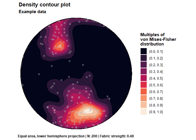
Density on a Sphere
Density shown by contour lines…
par(mfrow = c(1, 2))
contour(example_planes)
points(example_planes, col = "grey", cex = .5)
title(main = "Planes")

contour(example_lines)
points(example_lines, col = "grey", cex = .5)
title(main = "Lines")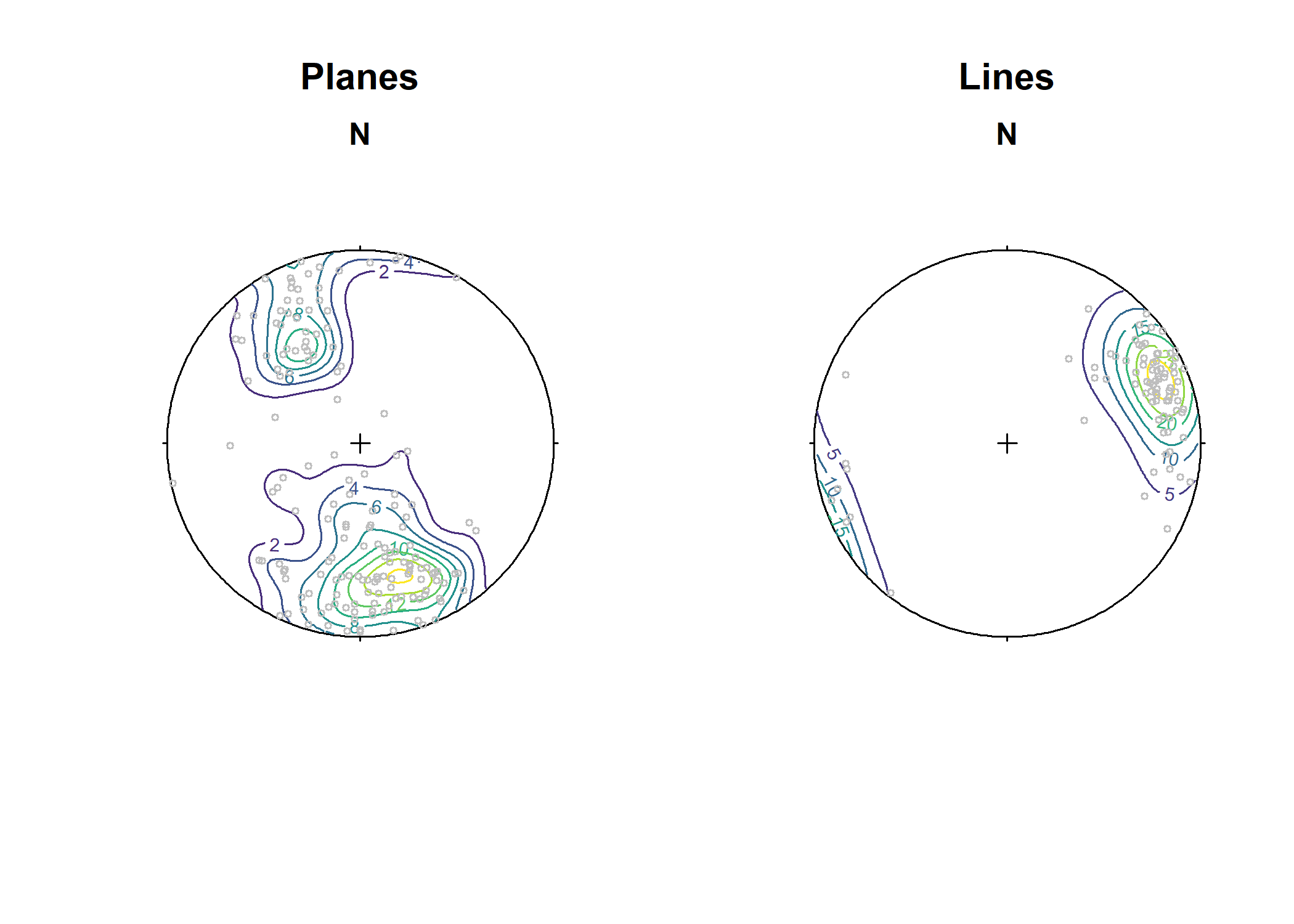
or as filled contours:
par(mfrow = c(1, 2))
image(example_planes)
points(example_planes, col = "grey", cex = .5)
title(main = "Planes")

image(example_lines)
points(example_lines, col = "grey", cex = .5)
title(main = "Lines")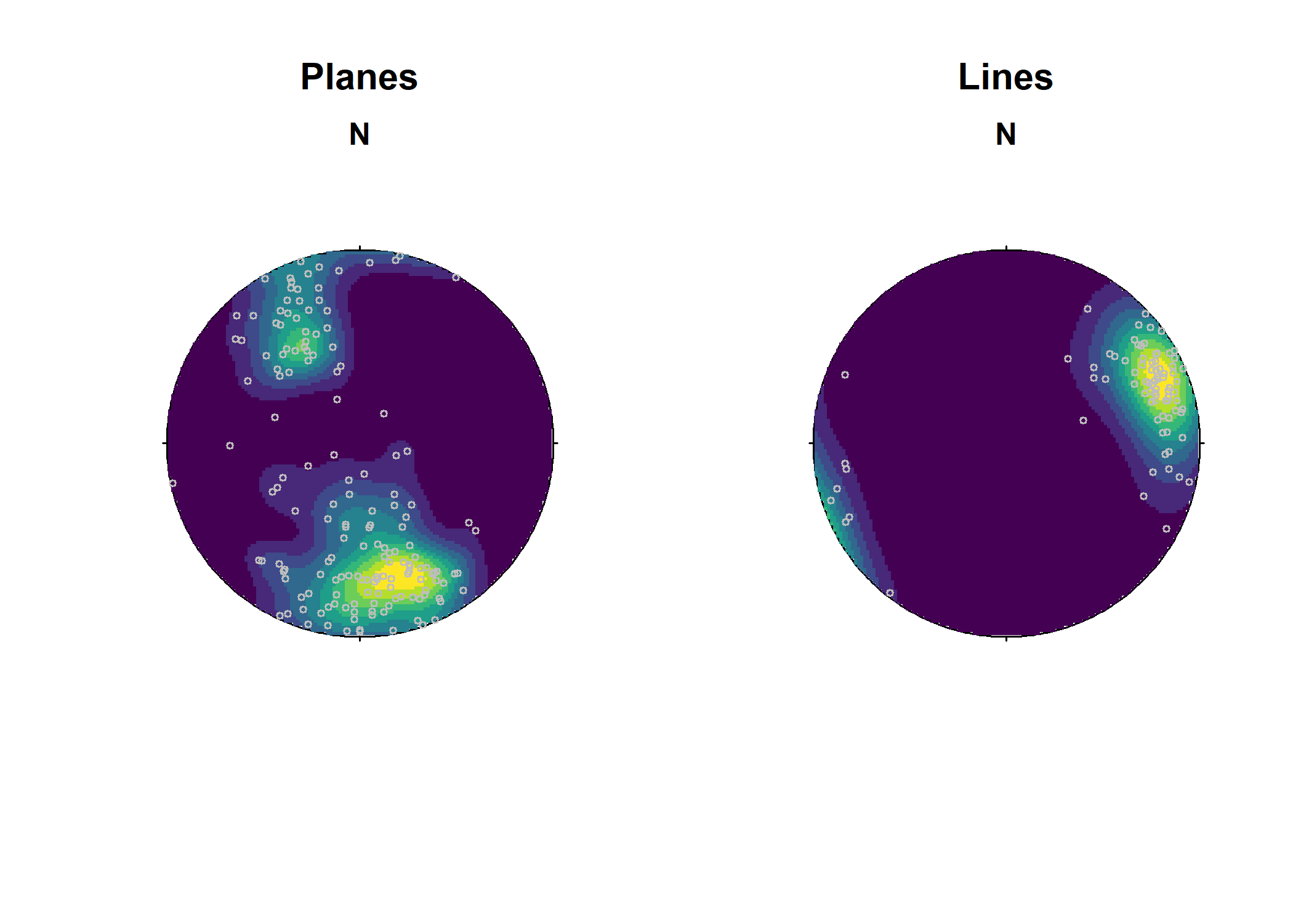
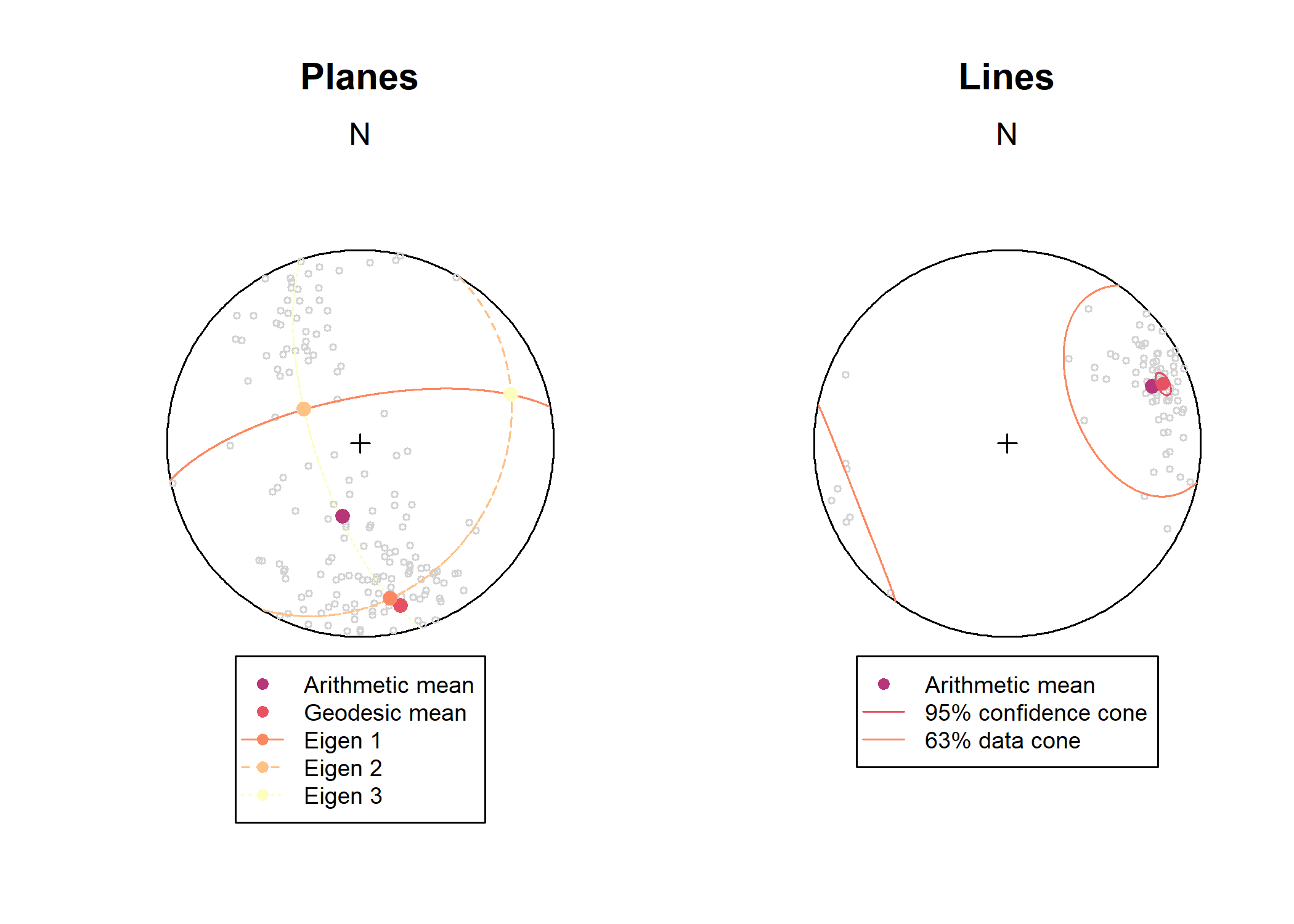
Spherical Statistics
Calculation of arithmetic mean, geodesic mean, confidence cones and eigenvectors… and plotting them in the equal-area projection:
planes_mean <- sph_mean(example_planes)
planes_geomean <- geodesic_mean(example_planes)
planes_eig <- ot_eigen(example_planes)$vectors

par(mfrow = c(1, 2), xpd = NA)
stereoplot(title = "Planes", guides = FALSE)
points(example_planes, col = "lightgrey", pch = 1, cex = .5)
lines(planes_eig, col = c("#FB8861FF", "#FEC287FF", "#FCFDBFFF"), lty = 1:3)
points(planes_mean, col = "#B63679", pch = 19, cex = 1)
points(planes_geomean, col = "#E65164FF", pch = 19, cex = 1)
points(planes_eig, col = c("#FB8861FF", "#FEC287FF", "#FCFDBFFF"), pch = 19, cex = 1)
legend(
  0, -1.1,
  xjust = .5,
  legend = c("Arithmetic mean", "Geodesic mean", "Eigen 1", "Eigen 2", "Eigen 3"),
  col = c("#B63679", "#E65164FF", "#FB8861FF", "#FEC287FF", "#FCFDBFFF"),
  pch = 19, lty = c(NA, NA, 1, 2, 3),
  cex = .75
)

lines_mean <- sph_mean(example_lines)
lines_delta <- delta(example_lines)
lines_confangle <- confidence_ellipse(example_lines)

stereoplot(title = "Lines", guides = FALSE)
points(example_lines, col = "lightgrey", pch = 1, cex = .5)
points(lines_mean, col = "#B63679", pch = 19, cex = 1)
stereo_confidence(lines_confangle, col = "#E65164FF")
lines(lines_mean, ang = lines_delta, col = "#FB8861FF")
legend(
  0, -1.1,
  xjust = .5,
  legend = c("Arithmetic mean", "95% confidence cone", "63% data cone"),
  col = c("#B63679", "#E65164FF", "#FB8861FF"),
  pch = c(19, NA, NA), lty = c(NA, 1, 1), cex = .75
)
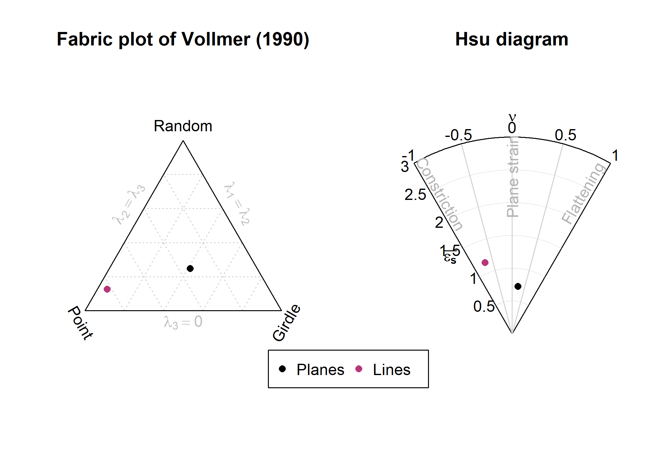
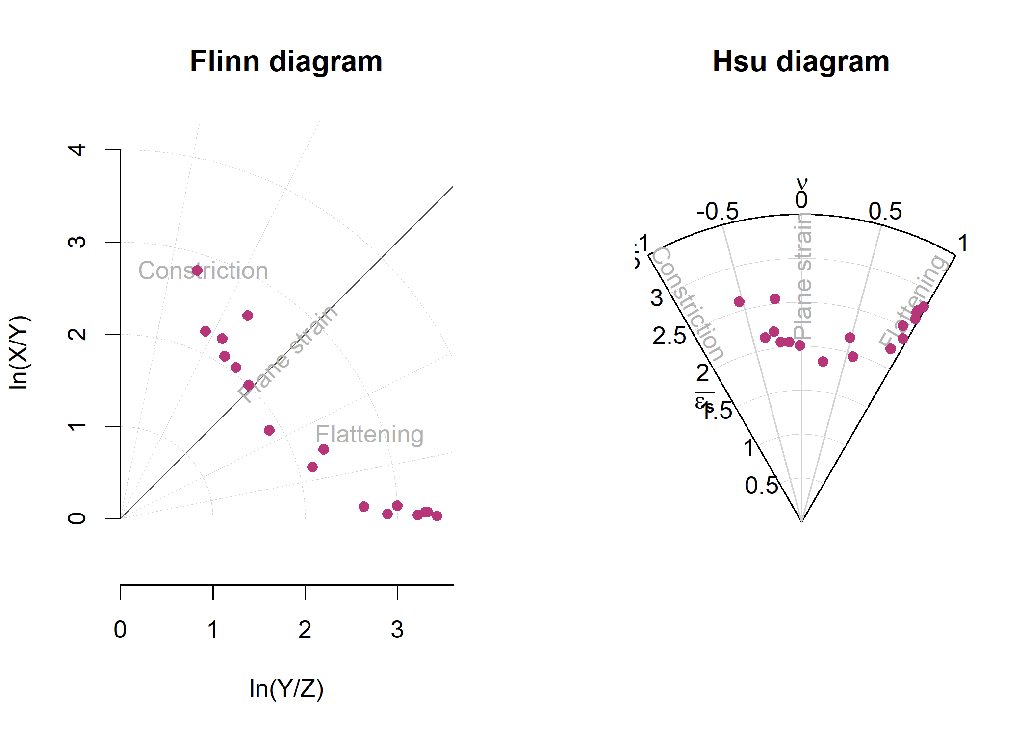
Orientation Tensor and Fabric Plots
The shape parameters of the orientation tensor of the above examples planes and lines can be visualized in two ways:
par(mfrow = c(1, 2), xpd = NA)
vollmer_plot(example_planes, col = "#000004", pch = 16)
vollmer_plot(example_lines, col = "#B63679FF", pch = 16, add = TRUE)

hsu_plot(example_planes, col = "#000004", pch = 16)
hsu_plot(example_lines, col = "#B63679FF", pch = 16, add = TRUE)

legend(
  2.5, -.25,
  xjust = .5, horiz = TRUE, xpd = NA,
  legend = c("Planes", "Lines"), col = c("#000004", "#B63679FF"), pch = 16
)
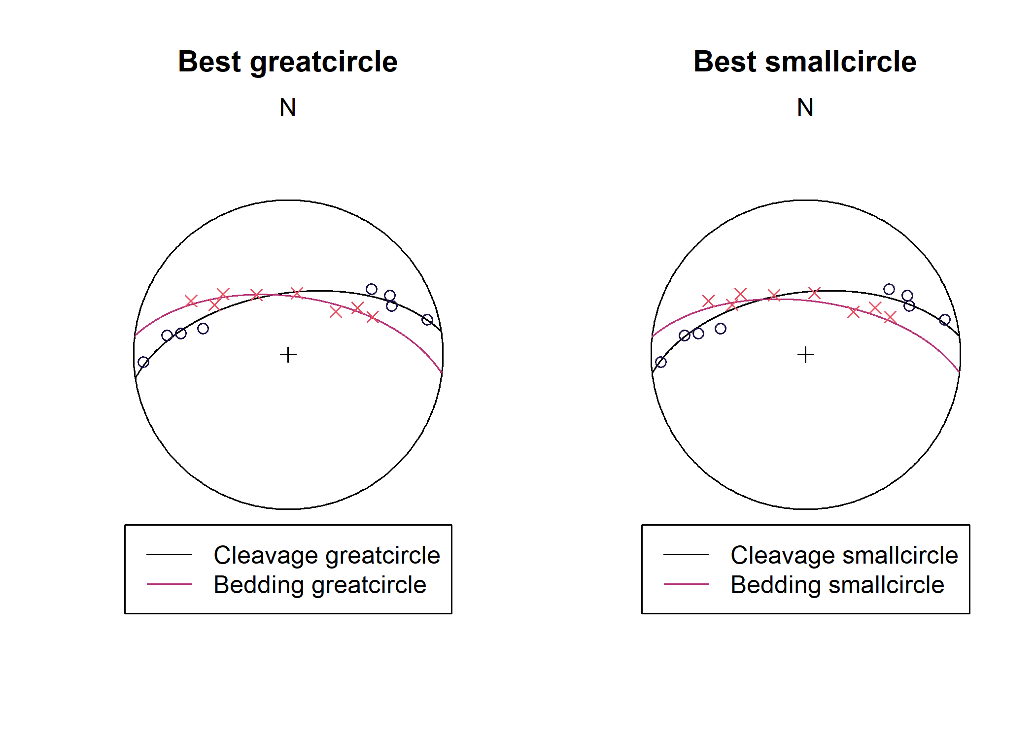
Best-fit Great- and Small-Circles (Geodesic Regression)
Finds the best-fit great or small-circle for a given set of vectors by applying geodesic regression:
set.seed(20250411)
data("gray_example")
cleavage <- gray_example[1:8, ]
bedding <- gray_example[9:16, ]

cleavage_gc <- regression_greatcircle(cleavage)
bedding_gc <- regression_greatcircle(bedding)

cleavage_sc <- regression_smallcircle(cleavage)
bedding_sc <- regression_smallcircle(bedding)

par(mfrow = c(1, 2), xpd = NA)
stereoplot(title = "Best greatcircle", guides = FALSE)
lines(cleavage_gc$vec, col = "#000004FF")
lines(bedding_gc$vec, col = "#B63679")
points(cleavage, col = "#1D1147")
points(bedding, col = "#E65164", pch = 4)

legend(
  0, -1.1,
  xjust = .5,
  col = c("#000004FF", "#B63679"),
  lty = c(1, 1), legend = c("Cleavage greatcircle", "Bedding greatcircle"), bg = "white"
)

stereoplot(title = "Best smallcircle", guides = FALSE)
lines(cleavage_sc$vec, cleavage_sc$cone, col = "#000004FF")
lines(bedding_sc$vec, bedding_sc$cone, col = "#B63679")
points(cleavage, col = "#1D1147")
points(bedding, col = "#E65164", pch = 4)

legend(0, -1.1,
  xjust = .5,
  col = c("#000004FF", "#B63679"), lty = c(1, 1), legend = c("Cleavage smallcircle", "Bedding smallcircle"), bg = "white"
)
Fault Plots
Graphical representation of fault-slip data using Angelier plot (slip vector on fault plane great circle) and Hoeppener plot (fault slip vector projected on pole to fault plane):
data("angelier1990")
faults <- angelier1990$TYM

par(mfrow = c(1, 2))
stereoplot(title = "Angelier plot", guides = FALSE)
angelier(faults, col = "grey20")

stereoplot(title = "Hoeppener plot", guides = FALSE)
hoeppener(faults, points = FALSE, col = "grey20")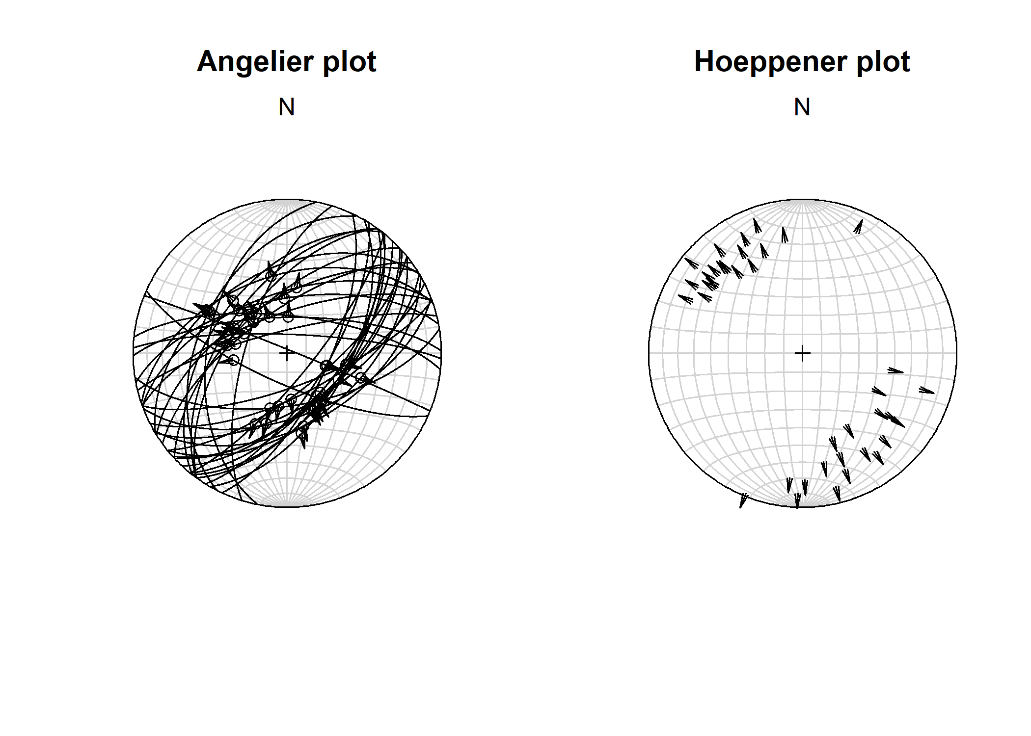
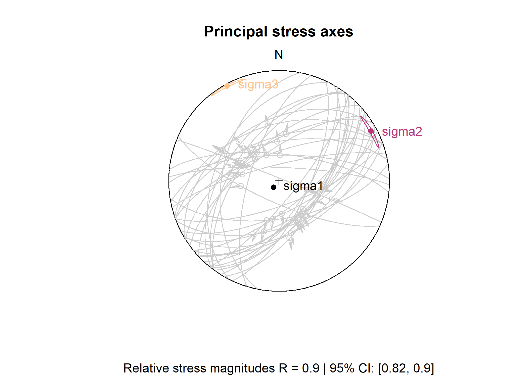
Fault-Slip Inversion
structr can calculate the reduced deviatoric stress tensor from fault-slip data using the direct inversion methods after Michael (1984), Angelier (1990), Yamajo & Sato (2006), and Hansen (2013). This allows to extract the orientation and relative magnitudes of the principal stress axes.
Here, we compute the reduced stress tensor using direct fault-slip inversion after Michael (1984) and calculate 95% confidence intervals using bootstrap replicates:
set.seed(20250411)
faults_stress <- slip_inversion(faults, n_iter = 10, method = 'michael')
Now we can visualize the slip inversion results, that are the orientation of principal stresses:
cols <- c("#000004FF", "#B63679FF", "#FEC287FF")
R_val <- round(faults_stress$stress_shape$R, 2)
R_CI <- round(faults_stress$R_CI, 2)

stereoplot(
  title = "Principal stress axes",
  sub = paste0("Relative stress magnitudes R = ", R_val, " | ", "95% CI: [", R_CI[1], ", ", R_CI[2], "]"),
  guides = FALSE
)
angelier(faults, col = "grey80")
stereo_confidence(faults_stress$principal_axes_CI$sigma1, col = cols[1])
stereo_confidence(faults_stress$principal_axes_CI$sigma2, col = cols[2])
stereo_confidence(faults_stress$principal_axes_CI$sigma3, col = cols[3])
text(faults_stress$principal_axes,
  label = rownames(faults_stress$principal_axes),
  col = cols, adj = -.25
)
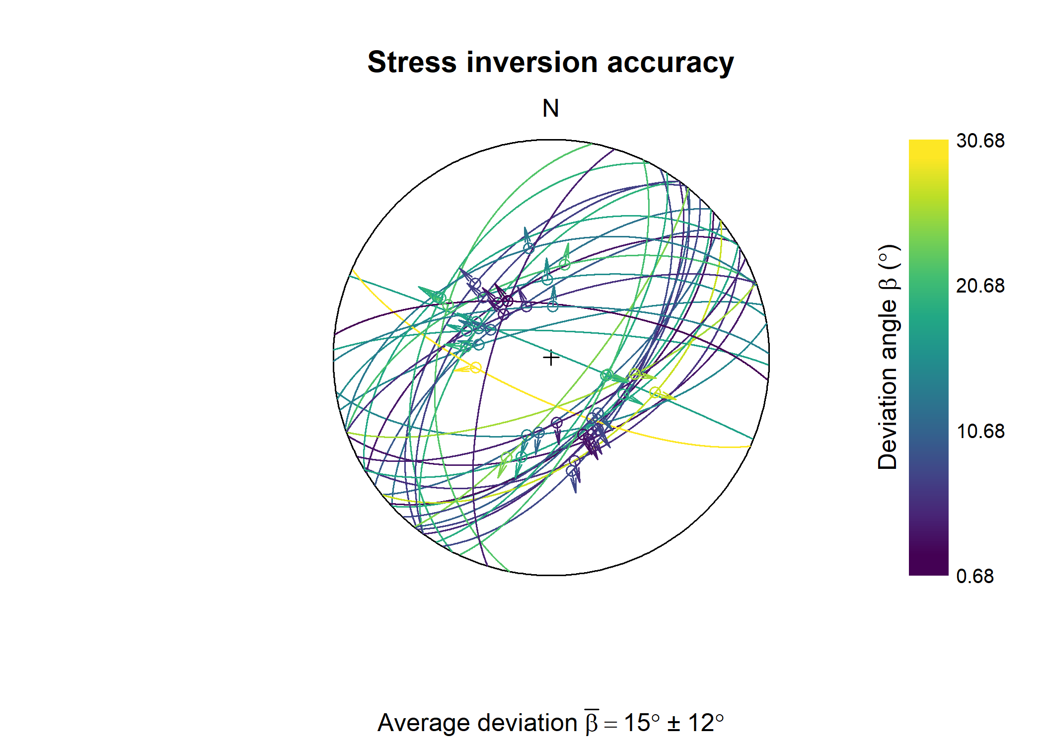
You can visualize the accuracy of the slip inversion by showing the deviation angle (α) between the theoretical slip and the actual slip vector:
alpha <- faults_stress$misfit$alpha
alpha_mean <- round(faults_stress$misfit$alpha_mean)
alpha_CI <- round(faults_stress$alpha_CI)

stereoplot(
  title = "Stress inversion accuracy",
  sub = bquote("Average deviation" ~ bar(alpha) == .(alpha_mean) * degree ~ "\U00B1" ~ .(alpha_CI) * degree),
  guides = FALSE
)
angelier(faults, col = assign_col(alpha))
legend_col(
  seq(min(alpha), max(alpha), 10),
  title = bquote("Deviation angle" ~ alpha ~ "(" * degree * ")")
)
The azimuth of the maximum horizontal stress (in degrees) for the slip inversion result is:
SH(
S1 = faults_stress$principal_axes[1, ],
S2 = faults_stress$principal_axes[2, ],
S3 = faults_stress$principal_axes[3, ],
R = faults_stress$stress_shape$R
)
#> [1] 60.80844
# or simply call
# faults_stress$SHmax
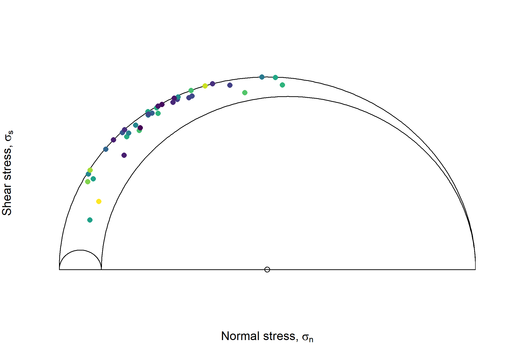
# faults_stress$SHmax_CI # confidence intervalMohr Circle
The Mohr circle for the slip inversion result can be visualized:
Mohr_plot(
  sigma1 = faults_stress$principal_vals[1],
  sigma2 = faults_stress$principal_vals[2],
  sigma3 = faults_stress$principal_vals[3],
  unit = NULL, include.zero = FALSE
)
points(faults_stress$stress_component[, 'normal'], abs(faults_stress$stress_component[, 'shear']),
  col = assign_col(alpha), pch = 16
)
Strain Analysis
2D Strain
Aspect ratio of finite strain ellipses vs orientation of long-axis (Rf/ϕ)
data(ramsay)

par(mfrow = c(1, 2))
Rphi_plot(r = ramsay[, 1], phi = ramsay[, 2])
elliott_plot(ramsay[, 1], ramsay[, 2], proj = "eqd")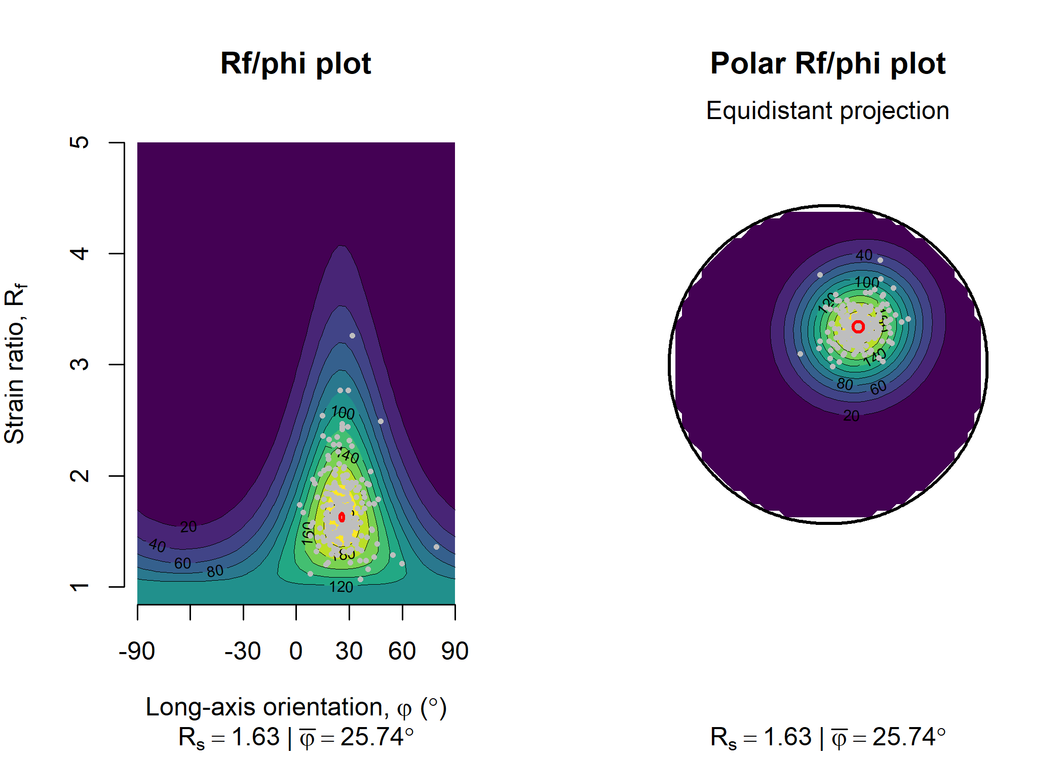
Vorticity Analysis
Aspect ratio of finite strain ellipses of porphyroclasts vs orientation of long-axis with respect to foliation plotted in the Rigid Grain Net
data(shebandowan)
set.seed(20250411)

# Color code porphyroclasts by size of clast (area in log-scale):
RGN_plot(shebandowan$r, shebandowan$phi, col = assign_col(log(shebandowan$area)), pch = 16)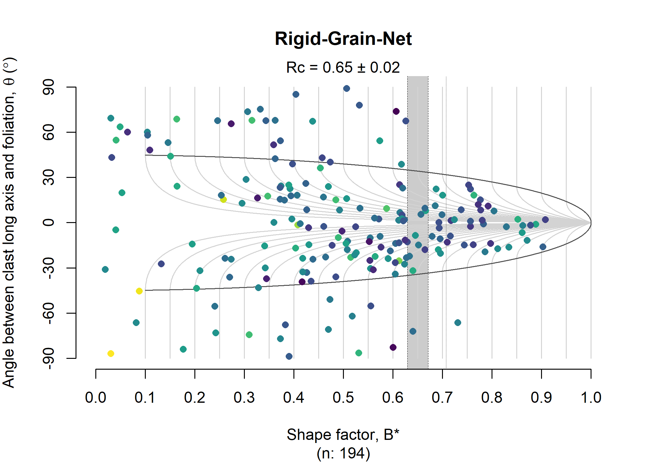
Deformation and Velocity Gradient Tensors
Define a deformation gradient tensor and deform some orientation data over time t in i increments:
# Define deformation time and increments
t <- 10
i <- 2

# Define deformation tensor:
D1 <- defgrad_from_generalshear(k = 2.5, gamma = 0.9)

# Generate some random lineation
xl <- rvmf(100, mu = Line(0, 90), k = 100)

# Generate the velcity gradient tensor for deformation accumulating over time
L <- velgrad(D1, time = t)

# Extract deformation increments
D1_steps <- defgrad(L, time = t, steps = i)

# Transform the lineation for each deformation increment
xl_steps <- lapply(D1_steps, function(i) {
  transform_linear(xl, i)
})

# instantaneous stretching axes
axes_ISA <- instantaneous_stretching_axes(L)

# flow apophyses
flow_apophyses <- flow_apophyses(L)

increments <- seq(0, t, i)

stereoplot(guides = FALSE)
stereo_path(xl_steps, type = "l")
stereo_path(xl_steps, type = "p", col = assign_col(increments), pch = 16, cex = .4)

lines(flow_apophyses, col = c("grey30", "grey70"), lty = c(1, 2))
points(axes_ISA, pch = 15, col = "#B63679FF")
text(axes_ISA, labels = c("ISA-1", "ISA-2", "ISA-3"), col = "#B63679FF", pos = 3, font = 2)

# legend
legend(0, -1.1,
  xjust = 0.5,
  legend = c("Flow apophysis 1", "Flow apophysis 2"),
  col = c("grey30", "grey70"),
  lty = c(1, 2)
)

legend_col(increments, title = "Time")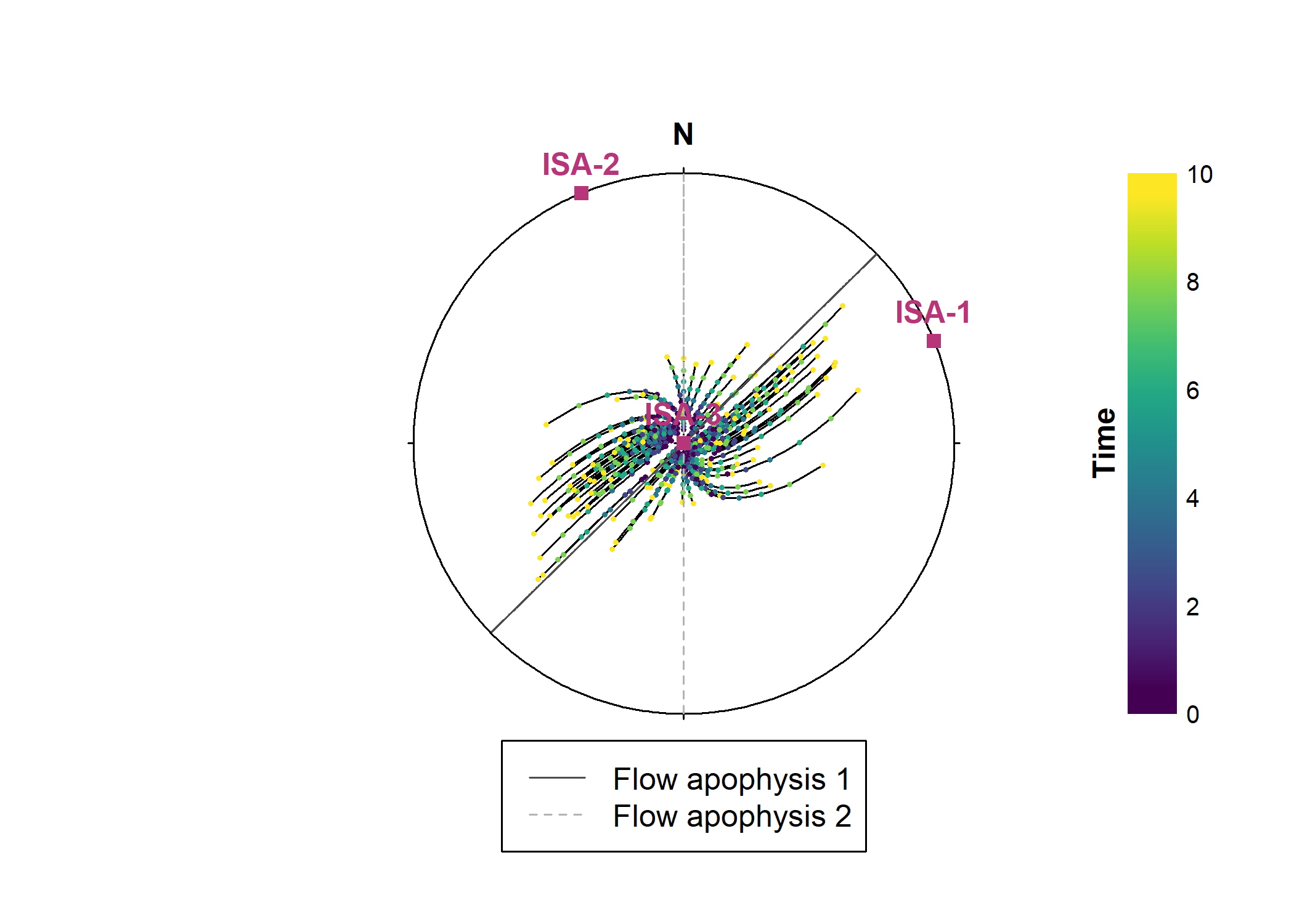
Show how the orientation tensor changes during progressive deformation:
par(mfrow = c(1, 2))
vollmer_plot(xl_steps, type = "b", col = assign_col(increments), pch = 16)
hsu_plot(xl_steps, type = "b", col = assign_col(increments), pch = 16)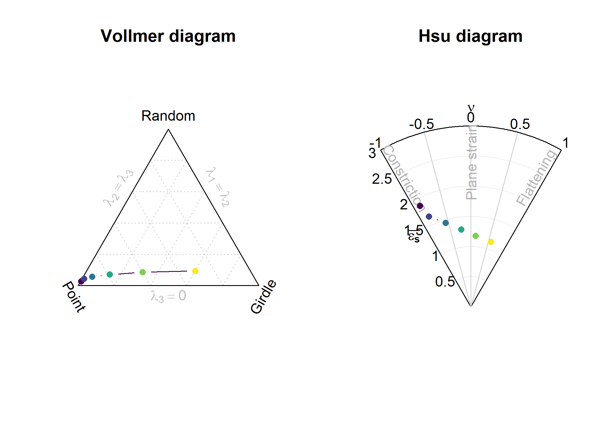
Author
Tobias Stephan (tstephan@lakeheadu.ca)
Feedback, issues, and contributions
I welcome feedback, suggestions, issues, and contributions! If you have found a bug, please file it here with minimal code to reproduce the issue.