Deformation and Velocity Gradient Tensor

This tutorial demonstrates how {structr} can be used to deform orientation data using deformation and velocity gradient tensors. This can be useful to simulate progressive deformation and change of orientation. It will also demonstrate how you can combine different deformation tensors, and how to extract other flow parameters (such as vorticity, stretching, and dilatation).

library(structr)

Deformation gradient tensor

3D deformation gradient tensor is a matrix that linearly transforms points. In other words it describes the changes of points in three dimensions.

Define a deformation gradient tensor

The deformation matrix can be defined using several ways:

defgrad_by_comp() creates an defined by individual components (default is identity tensor)
defgrad_by_ratio() creates an isochoric tensor with axial stretches defined by strain ratios (default is identity tensor).
defgrad_from_vectors() creates tensor representing rotation around the axis perpendicular to both vectors and rotate v1 to v2.
defgrad_from_axisangle() creates tensor representing a rigid-body rotation about an axis and an angle.
defgrad_from_pureshear() creates an isochoric coaxial tensor.
defgrad_from_simpleshear() creates an isochoric non-coaxial tensor.
defgrad_from_generalshear() creates an isochoric tensor, where transtension is $k>1$ and $\gamma \neq 0$ , and transpression is $k<1$ and $\gamma \neq 0$ (¹)
defgrad_from_dilation() creates tensor representing the volume change in z-direction.

D1 <- defgrad_from_generalshear(k = 2.5, gamma = 0.9)
print(D1)
#> Deformation gradient tensor
#>      [,1]     [,2] [,3]
#> [1,]    1 1.473332  0.0
#> [2,]    0 2.500000  0.0
#> [3,]    0 0.000000  0.4

Matrix algebra

An isochoric deformation tensor creates deformation without volume change. In that case, the determinant of the matrix must be 1. In R, this can be checked using det():

det(D1)
#> [1] 1

The inverse of the tensor reverses the deformation. In R, this can be done using solve():

solve(D1)
#>      [,1]       [,2] [,3]
#> [1,]    1 -0.5893326  0.0
#> [2,]    0  0.4000000  0.0
#> [3,]    0  0.0000000  2.5

The eigenvectors of the tensor describe the orientation of the strain ellipse, and the eigenvalues $\lambda$ describe its shape (i.e. length of the principal axes is proportional to the amount of stretch).

eigen(D1)
#> eigen() decomposition
#> $values
#> [1] 2.5 1.0 0.4
#> 
#> $vectors
#>           [,1] [,2] [,3]
#> [1,] 0.7007364    1    0
#> [2,] 0.7134203    0    0
#> [3,] 0.0000000    0    1

Deformation tensors can be combined using matrix multiplication. The resulting deformation from our general-shear deformation (D1) superimposed by our rotation (D2) is

D2 <- defgrad_from_axisangle(Line(0, 90), 30)

D12 <- D2 %*% D1 # D1 is applied first

Matrix multiplication is not commutative, i.e. $D1 \cdot D2 \neq D2 \cdot D1$

Transformation using deformation gradient tensor

The deformation can now be applied on some orientation data using linear transformation:

# generate some random lineation
xl <- rvmf(100, mu = Line(0, 90), k = 100)

xl_transformed <- transform_linear(xl, D1)
head(xl_transformed)
#> Vector (Vec3) object (n = 6):
#>                x           y         z
#> [1,] -0.10284016  0.04850097 0.3964546
#> [2,]  0.13775532  0.31523476 0.3963421
#> [3,]  0.04318670  0.24232166 0.3961172
#> [4,] -0.12970895 -0.33532970 0.3954535
#> [5,] -0.23446654 -0.31984836 0.3962864
#> [6,] -0.08260559  0.09628880 0.3957975

Let’s visualize the deformation:

# The coordinate axes of our deformation tensor:
axes <- Vec3(c(1, 0, 0), c(0, 1, 0), c(0, 0, 1))

stereoplot(guides = FALSE) # turn off guidelines for better visibility
points(xl, col = "grey", pch = 16)
points(xl_transformed, col = "#B63679FF", pch = 16)
points(axes, pch = 15)
text(axes, labels = c("x", "y", "z"), pos = 1, font = 3)

legend("right", legend = c("D0", "D1"), col = c("grey", "#B63679FF"), pch = 16)

Velocity gradient tensor

The velocity gradient tensor L describes the velocity of particles at any instant during the deformation. Velocity gradient tensor from deformation gradient tensor.

The time argument specifies the time of deformation, i.e. how many times the Deformation gradient tensor should be applied.

L <- velgrad(D1, time = 10)

Decomposition

The velocity gradient tensor L can be decomposed into a symmetric matrix S (the strain rate or stretching tensor) and the skew-symmetric matrix W (the spin tensor).

The stretching matrix (or tensor) and describes the portion of the deformation that over time produces strain:

S <- velgrad_rate(L)

The spin tensor contains information about the internal rotation during the deformation:

W <- velgrad_spin(L)

The eigenvectors of the stretching gradient tensor give the orientations and lengths of the instantaneous stretching axes:

S_eig <- eigen(S)

# ISA vectors
axes_ISA <- S_eig$vectors |>
  as.Vec3() |>
  Line()

# Amounts of stretching
S_eig$values
#> [1]  0.11003269 -0.01840362 -0.09162907

The shortcut functions instantaneous_stretching_axes(L) and instantaneous_stretching(L) produce the same results as above.

The eigenvectors of the velocity gradient tensor describe the flow apophyses:

L_eig <- eigen(L)

# Flow apophyses
flow_vectors <- L_eig$vectors |>
  t() |>
  as.Vec3()

flow_apophyses <- rbind(
  crossprod(flow_vectors[1, ], flow_vectors[2, ]),
  crossprod(flow_vectors[2, ], flow_vectors[3, ])
) |> Plane()

short cut: flow_apophyses(L)

The angle α between the apophyses is directly related to how close to simple shear or pure shear the deformation is. α is zero for simple shear and 90° for pure shear. The kinematic vorticity number $W_k$ is given by $W_k = \cos\alpha$ :

alpha <- angle(flow_apophyses[1, ], flow_apophyses[2, ])
abs(cos(alpha * pi / 180))
#> [1] 0.7007364

short cut: kinematic_vorticity_from_velgrad(L)

The vorticity vector is the eigenvector corresponding to the intermediate eigenvalue of the velocity gradient tensor:

Line(flow_vectors[2, ])
#> Line object (n = 1):
#> azimuth  plunge 
#>       0      90

shortcut: vorticity_vector(L)

Strain increments

Now we can extract the deformation gradient tensor accumulated after a given time. Here we extract the deformation gradient tensors for some time steps using defgrad()

The steps argument specifies how many increments you would like to extract (this is also is the “resolution” of the deformation path)
The time

D1_steps <- defgrad(L, time = 10, steps = 2)

Now apply the deformation tensors on some orientation data

xl_steps <- lapply(D1_steps, function(i) {
  transform_linear(xl, i)
})

Visualization of deformation over time

And plot the paths showing how the orientations change over time

increments <- seq(0, 10, 2)
cols <- assign_col(increments)

stereoplot(guides = FALSE) # turn off guidelines for better visibility

# plot the strain increments
stereo_path(xl_steps, type = "l")
stereo_path(xl_steps, type = "p", col = cols, pch = 16, cex = .4)

# flow apophyses
lines(flow_apophyses, col = c("grey30", "grey70"), lty = c(1, 2))

# instantaneous stretching axes
points(axes_ISA, pch = 15, col = "#B63679FF")
text(axes_ISA, labels = c("ISA-1", "ISA-2", "ISA-3"), col = "#B63679FF", pos = 3, font = 2)

# coordinate axes of def-tensor
points(axes, pch = 15)
text(axes, labels = c("x", "y", "z"), pos = 1, font = 3)

# legend
legend(0, -1.1,
  xjust = 0.5,
  legend = c("Flow apophysis 1", "Flow apophysis 2"),
  col = c("grey30", "grey70"),
  lty = c(1, 2)
)
legend_c(increments, title = "Time")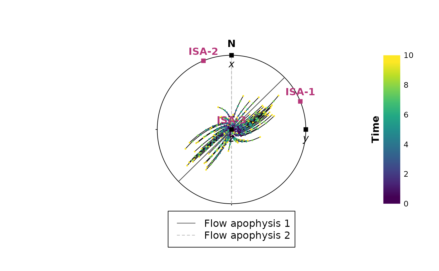

We can also monitor how the orientation tensor changes during progressive deformation:

par(mfrow = c(1, 2))
vollmer_plot(xl_steps, type = "b", col = cols)
hsu_plot(xl_steps, type = "b", col = cols)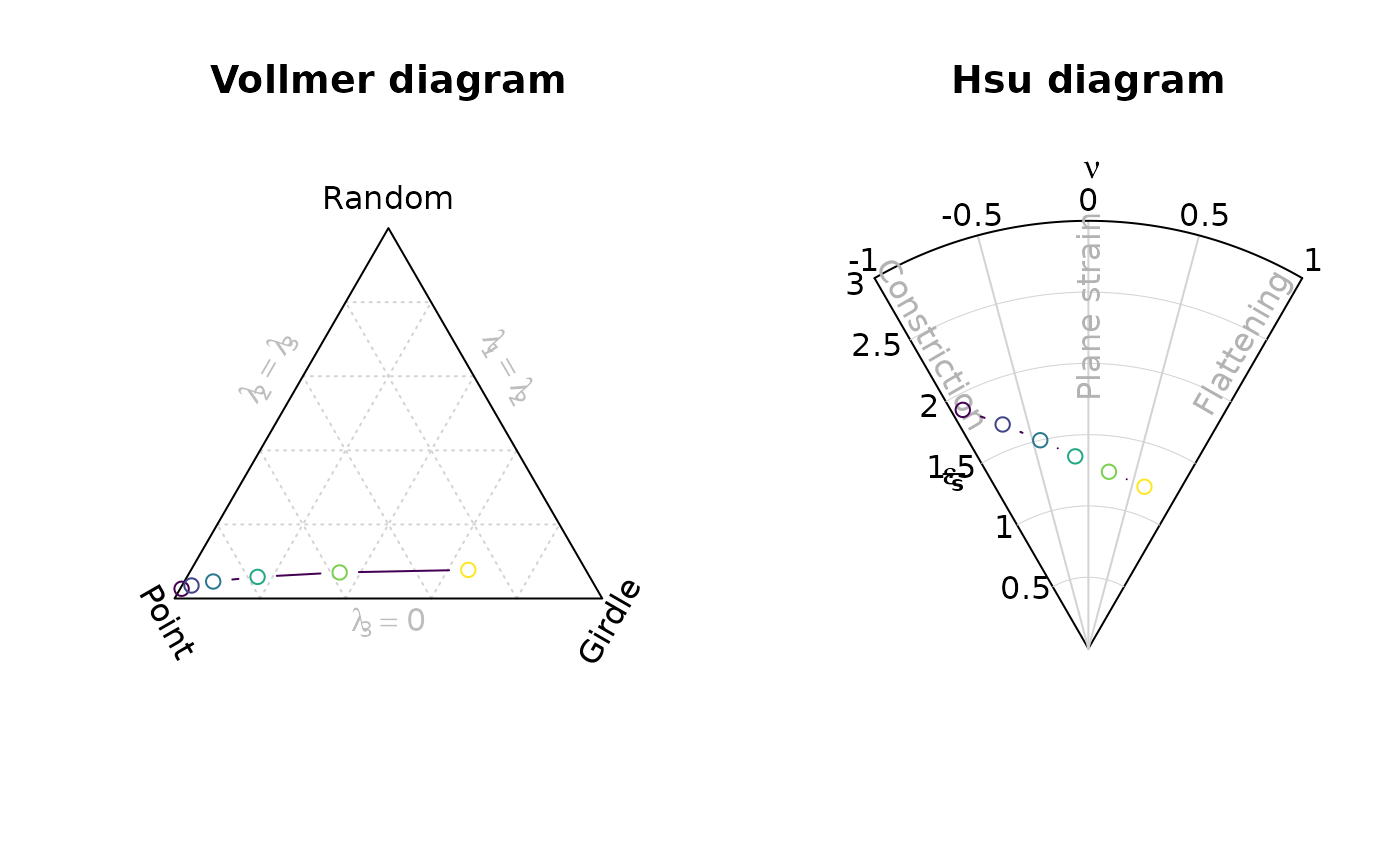

References

Fossen, H., & Tikoff, B. (1993). The deformation matrix for simultaneous simple shearing, pure shearing and volume change, and its application to transpression-transtension tectonics. Journal of Structural Geology, 15(3–5), 413–422. https://doi.org/10.1016/0191-8141(93)90137-Y

Sanderson, D. J., & Marchini, W. R. D. (1984). Transpression. Journal of Structural Geology, 6(5), 449–458. https://doi.org/10.1016/0191-8141(84)90058-0

Tobias Stephan

2025-11-06