This tutorial describes how to calculate basic statistics for spherical orientation data using the structr package. It covers the calculation of mean orientations, dispersion measures, hypothesis testing, orientation tensors, and clustering of orientation data.
Load the package:
To start, we import some example planes and lines, and convert them to spherical objects:
data(example_planes_df)
data(example_lines_df)

planes <- Plane(example_planes_df$dipdir, example_planes_df$dip)
lines <- Line(example_lines_df$trend, example_lines_df$plunge)
Mean and Dispersion
Arithmetic mean, geodesic mean, and projected mean
Arithmetic Mean and Variance
The arithmetic mean orientation of spherical data is calculated by summing up all orientation vectors and normalizing the resulting vector1:
This involves the resultant vector of a set of vectors , given by , and the resultant length defined as .
The arithmetic mean of the vector components is the mean resultant vector, i.e the resultant vector normalized by its length
In geology, the statistical estimators are useful for
vectorial data ("Line" objects) such as
lineations (e.g. mineral lineations, stretching lineations) or plunge
directions of fold axes, but less for axial data ("Ray"
objects) such as paleomagnetic directions or orientations of fold axes,
where the direction is not relevant2.
These estimators are good descriptors of the concentration of the data around the mean direction, assuming an unimodal, isotropic distributions such as the von Mises-Fisher distribution.
Define some weights for our lines based on the quality reported for the measurements:
example_lines_df$quality <- ifelse(is.na(example_lines_df$quality), 1, example_lines_df$quality) # replacing NA values with 1
line_weightings <- 5 / example_lines_df$quality
The (weighted) arithmetic mean orientation of spherical data is:
lines_mean <- sph_mean(lines, w = line_weightings)… and the (weighted) arithmetic variance
lines_variance <- sph_var(lines, w = line_weightings)the (weighted) standard deviation (i.e. the 63% cone around the mean) and the 95% confidence cone around the mean:
lines_delta <- delta(lines, w = line_weightings)
lines_confangle <- sph_confidence_angle(lines, w = line_weightings)
Taken together, this prints as
c(
  "Variance" = lines_variance,
  "63% cone" = lines_delta,
  "Confidence angle" = lines_confangle
)
#>         Variance         63% cone Confidence angle
#>        0.1568745       32.5283448        6.6748765
Summary stats can also be retrieved through
summary(lines)
#>         azimuth          plunge        variance        68% cone confidence cone
#>      68.5127690      20.4958671       0.2168518      38.4502642       4.7492331
Plotting a summary of the stats on a equal-area projection:
stereoplot(center  = lines_mean)
points(lines, col = "lightgrey", pch = 1, cex = .5)
points(lines_mean, col = "#B63679", pch = 19, cex = 1)
lines(lines_mean, ang = lines_confangle, col = "#E65164FF")
lines(lines_mean, ang = lines_delta, col = "#FB8861FF")
legend("topright", legend = c("Mean line", "95% confidence cone", "63% data cone"), col = c("#B63679", "#E65164FF", "#FB8861FF"), pch = c(19, NA, NA), lty = c(NA, 1, 1), cex = .75)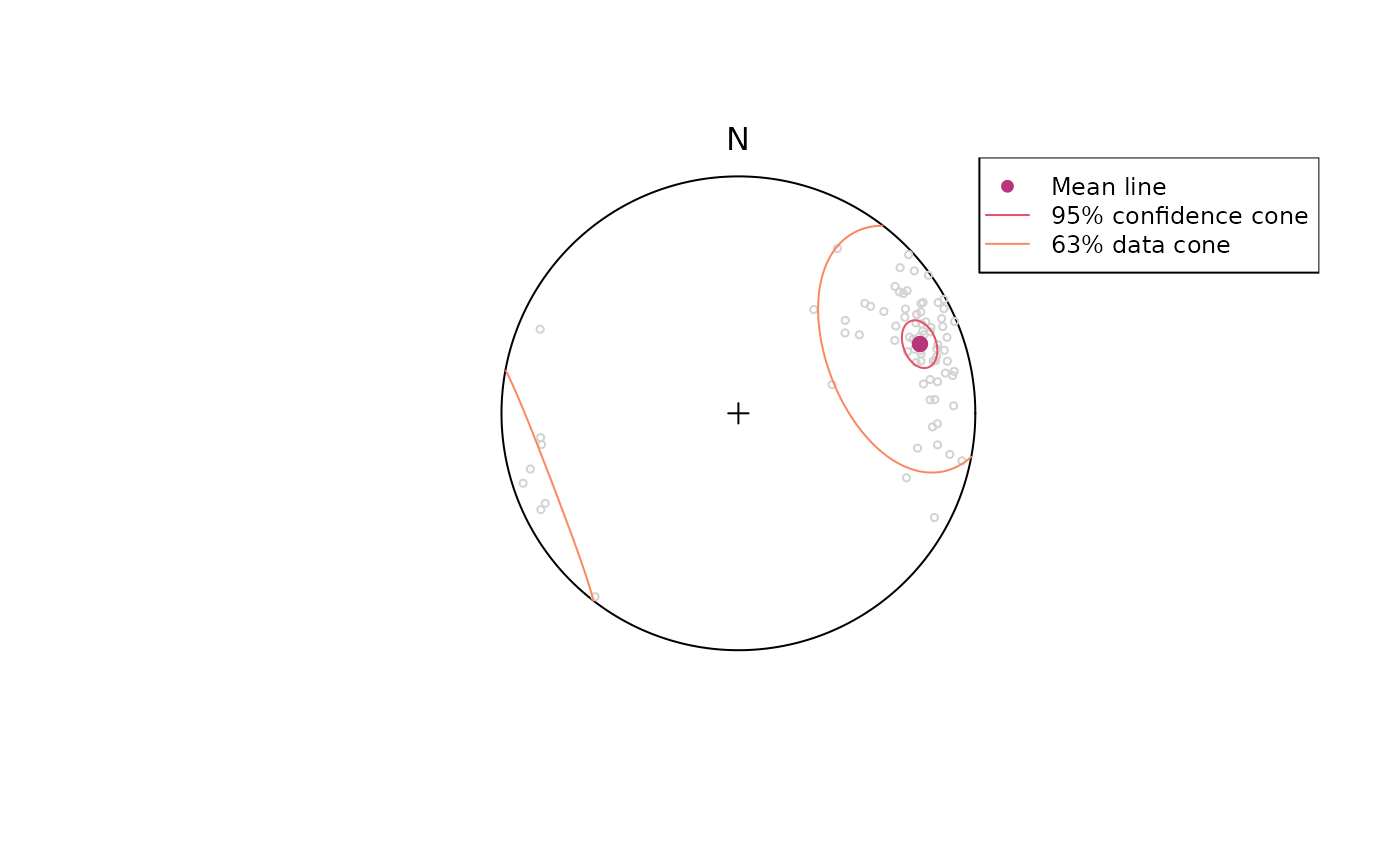
Geodesic Mean and Variance
Another measure of mean and dispersion is the Fréchet (geodesic
L2) mean and variance which is based on the
angles between all data vectors3.
This can be visualized using the variance_plot(); here
showing the (geodesic) angle distances between all lines and the first
line in the same data set:
variance_plot(lines, y = lines[1, ])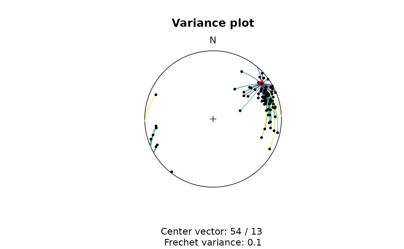
The Fréchet mean is the vector that minimizes the sum of the squared angle distances to all data vectors. The Fréchet variance about this mean is the sum of the squared angle distances between all data vectors and the Fréchet mean.
To find the Fréchet mean vector, the algorithm iteratively searches for the vector by using a numerical optimization method to minimize the distances to all other vectors
# Mean
geodesic_mean(lines)
#> Line object (n = 1):
#>  azimuth   plunge
#> 69.64061 14.87921

# Variance
geodesic_var(lines)
#> [1] 0.06118261
These estimators are good descriptors of the concentration of the data around the mean direction, when data follows a unimodal, anisotropic distributions such as the Kent or Bingham distributions.
Projected Mean
The Eigenvector with the largest Eigenvalue represents a vector parallel to the highest concentration of a population. This vector can also be described as the projected mean. A shortcut function for this is:
projected_mean(example_lines)
#> Line object (n = 1):
#>  azimuth   plunge
#> 69.09796 14.82125
These estimators are good descriptors of the concentration of the data around the mean direction, when data follows an unimodal, anisotropic distributions such as the Kent or Bingham distributions.
par(mfrow = c(1, 2))
stereoplot(center = sph_mean(example_lines))
points(example_lines, col = "grey", pch = 16, cex = .7)
points(sph_mean(example_lines), col = "#1D1147FF", pch = 16)
points(geodesic_mean(example_lines), col = "#B63679FF", pch = 16)
points(projected_mean(example_lines), col = "#FEC287FF", pch = 16)
title(main = "Lines")

legend("bottomleft",
  legend = c("Arithmetic mean", "Geodesic mean", "Projected mean"),
  col = c("#1D1147FF", "#B63679FF", "#FEC287FF"),
  pch = 16,
  bg = "white"
)

stereoplot(center = sph_mean(example_lines))
points(example_planes, col = "grey", pch = 16, cex = .7)
points(sph_mean(example_planes), col = "#1D1147FF", pch = 16)
points(geodesic_mean(example_planes), col = "#B63679FF", pch = 16)
points(projected_mean(example_planes), col = "#FEC287FF", pch = 16)
title(main = "Planes")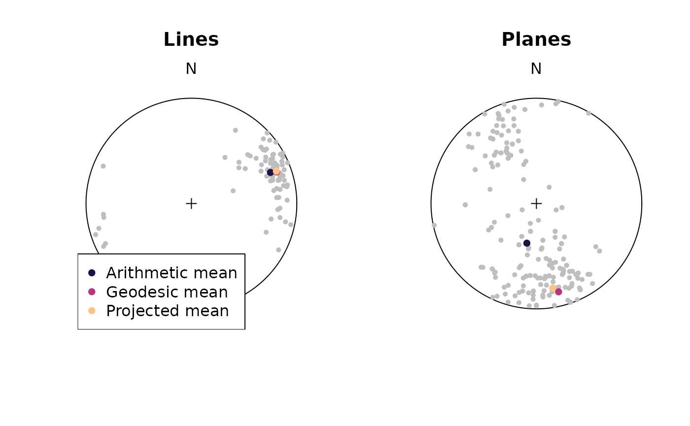
Orientation Tensor
Eigenvectors
The orientation tensor4 is a matrix comprising the mean direction cosines of the orientation vectors. In case of a Bingham distribution, the Eigenvectors of this tensor describe the orientation of the most dense, intermediate and least dense orientation, and thus, are used to determine the orientation of girdle-distributed vectors (e.g. folded planes).
The orientation tensor of orientation tensor is calculated by
ortensor():
ortensor(planes)
#> Orientation tensor
#>            [,1]        [,2]        [,3]
#> [1,]  0.5634412 -0.11043381 -0.12507927
#> [2,] -0.1104338  0.13269479 -0.04040902
#> [3,] -0.1250793 -0.04040902  0.30386403
The Eigenvalues from orientation data can be computed through
ot_eigen()
planes_eigen <- ot_eigen(planes)
print(planes_eigen)
#> eigen() decomposition
#> $values
#> [1] 0.62975929 0.28812045 0.08212026
#>
#> $vectors
#> Line object (n = 3):
#>        azimuth   plunge
#> [1,] 169.08091 19.46169
#> [2,] 300.98901 62.11934
#> [3,]  72.03016 19.15562
To visualize the orientation of the Eigenvectors and their -values,
you can call the vectors and values of the object returned by
ot_eigen():
stereoplot(center = planes_eigen$vectors[3, ])
points(example_planes, col = "grey", pch = 16, cex = .7)
lines(planes_eigen$vectors,
       col = c("#000004", "#B63679FF", "#FEC287FF"),
       lwd = rev(assign_cex(planes_eigen$values, range = c(.5, 2))))
points(planes_eigen$vectors,
       col = c("#000004", "#B63679FF", "#FEC287FF"),
       cex = assign_cex(planes_eigen$values, range = c(.5, 2)),
       pch = 16)
legend('right',
       legend = c("Eigen-1", "Eigen-2", "Eigen-3"),
       col = c("#000004", "#B63679FF", "#FEC287FF"), pch = 16, lty = 1)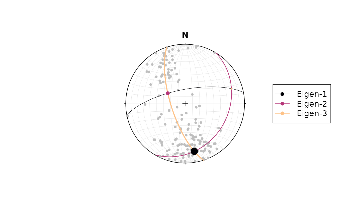
Shape Parameters
There are more shape parameters using different algorithms based on the orientation tensor:
shape_params(planes)
#> $stretch_ratios
#>      Rxy      Ryz      Rxz
#> 1.478428 1.873104 2.769250
#>
#> $strain_ratios
#>       e12       e13       e23
#> 0.3909795 1.0185765 0.6275970
#>
#> $Flinn
#> $Flinn$k
#> [1] 0.5479625
#>
#> $Flinn$d
#> [1] 0.9955924
#>
#>
#> $Ramsay
#> intensity  symmetry
#> 0.5467429 0.6229787
#>
#> $Woodcock
#>  strength     shape
#> 1.0185765 0.6229787
#>
#> $Watterson_intensity
#> [1] 2.351532
#>
#> $Lisle_intensity
#> [1] 1.147654
#>
#> $Nadai
#>      goct      eoct
#> 0.8391109 0.7266914
#>
#> $Lode
#> [1] 0.2323021
#>
#> $kind
#> [1] "SSL"
#>
#> $MAD
#> [1] 32.80303
#>
#> $Jelinek
#> [1] 2.794622
Maximum Likelihood Estimation of Distribution Parameters
par(mfrow = c(2, 2), mar = c(2, 2, 1, 1))
x1 <- rvmf(100, mu = Ray(120, 50), k = 5)
r1 <- fisher_MLE(x1)
plot(x1, col = 'grey')
points(r1$muHat, col = 'red')
title(main = 'von Mises-Fisher')

x2 <- rwatson(100, mu = Line(120, 50), k = 5)
r2 <- watson_MLE(x2)
plot(x2, col = 'grey')
points(r2$muHat, col = 'red')
title(main = 'Watson')

x3 <- rkent(100, mu = Ray(120, 50), k = 5, b = 1)
r3 <- kent_MLE(x3)
plot(x3, col = 'grey')
points(r3$G, col = 'red')
title(main = 'Kent')

a <- cov(iris[, 1:3])
x4 <- rbingham(100, a, "Line")
r4 <- bingham_MLE(x4)
plot(x4, col = 'grey')
points(r4$vectors, col = 'red')
title(main = 'Bingham')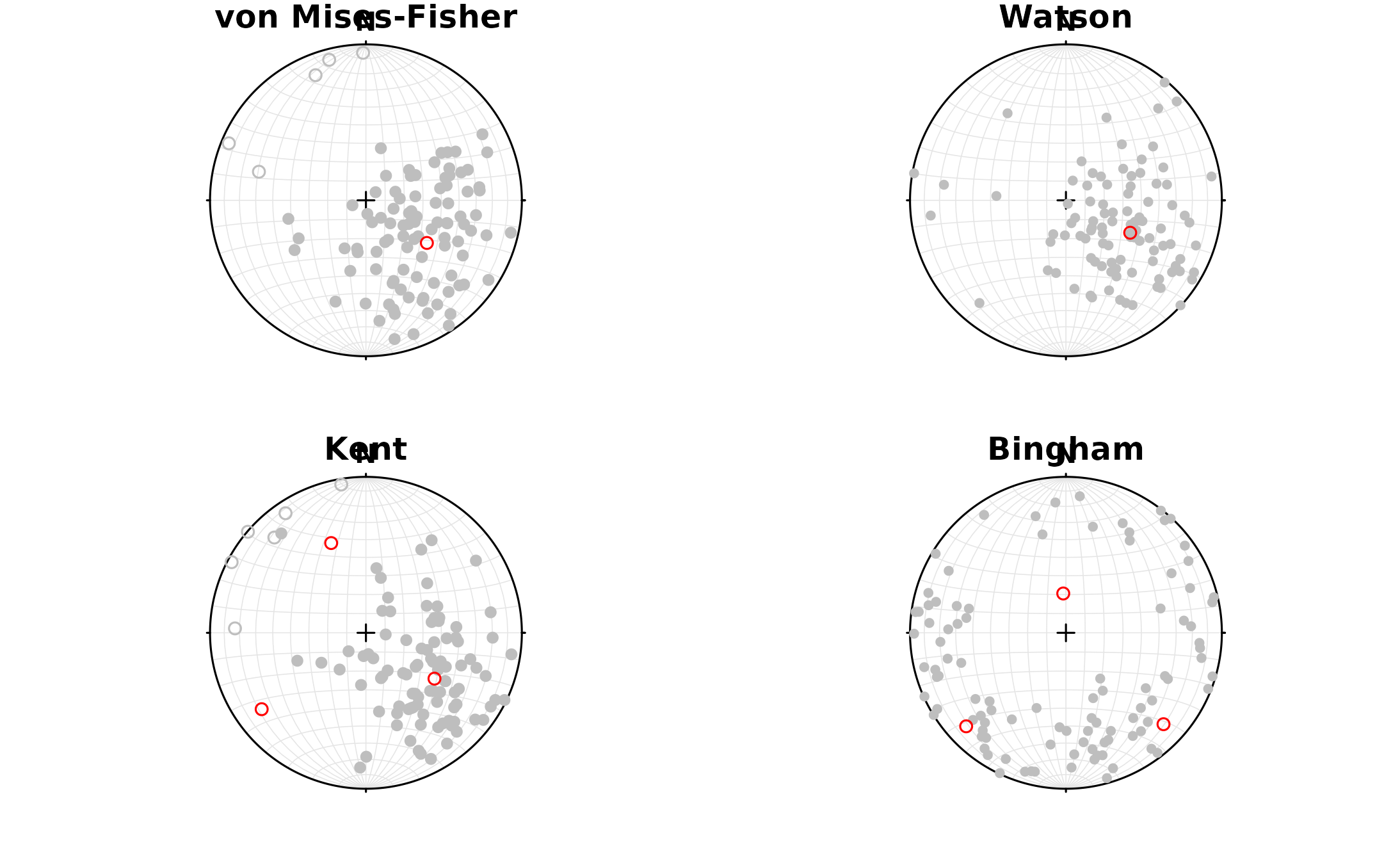
Hypothesis Testing
To test if a line represents the population mean of a given set of lineations, we need to calculate the confidence region of our population.
Let’s test the hypothesis that a horizontal lineation trending towards 70° is the mean for our lineations.
line_NULL <- Line(2, 10)Parametric Testing
Parametric testing means that we assume a specific underlying distribution of the data. Here, we assume that the lineations are drawn from a von Mises-Fisher distribution.
Confidence Region
cep <- fisher_inference(lines, alpha = 0.05)
plot(lines, col = "grey")
points(cep$muHat, col = "#B63679FF", pch = 16)
lines(cep$muHat, ang = cep$angle, col = "#B63679FF")
points(line_NULL, col = "#000004", pch = 16)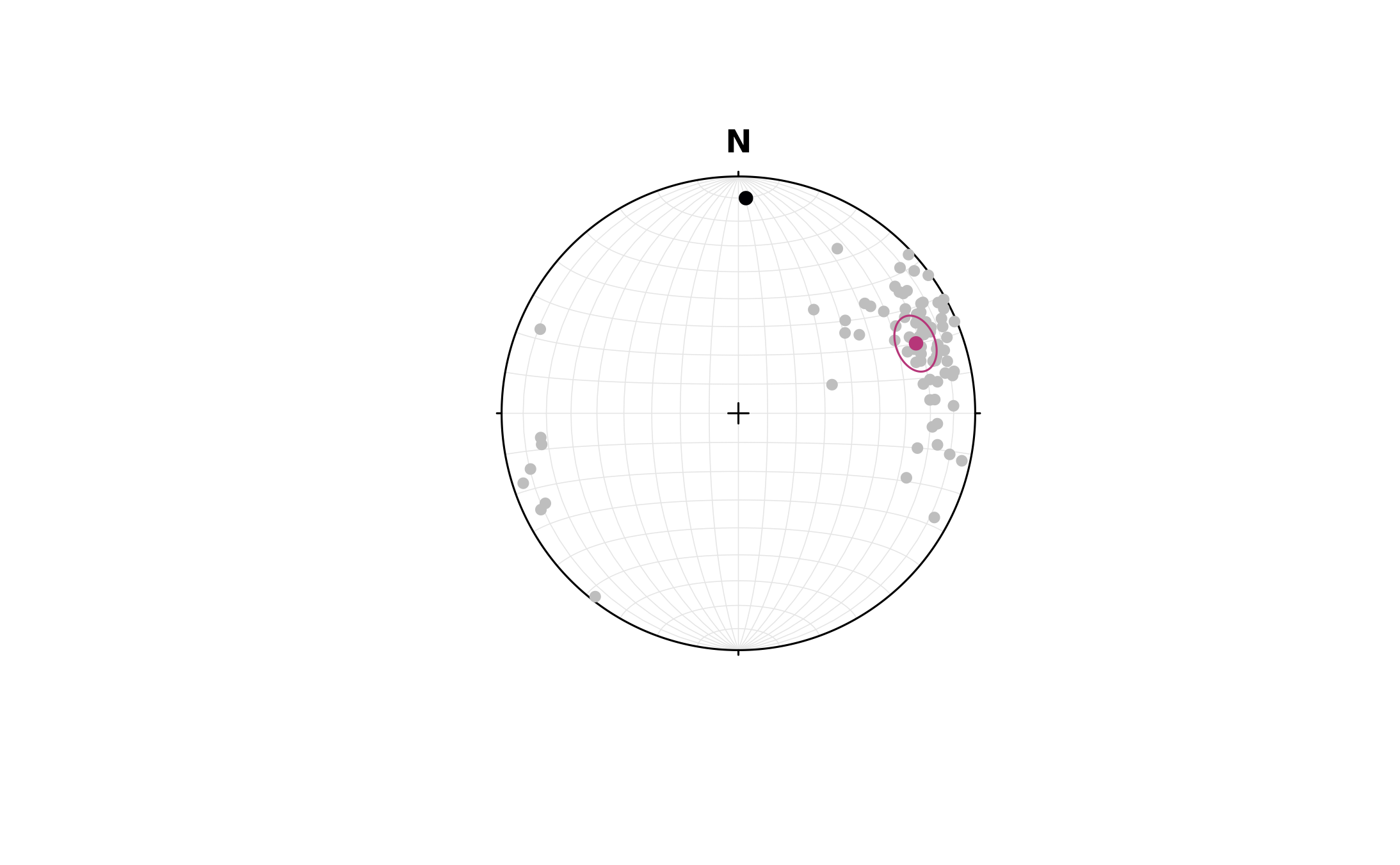
Non-parametric Testing
Non-parametric testing does require assumptions on the distribution of the data. This is commonly achieved using bootstrapping and permutation techniques.
Confidence Region
The 95% confidence interval (from 10,000 bootstrap samples):
cenp <- confidence_ellipse(lines, n = 10000, alpha = 0.05)To visualize the confidence region of our lines:
plot(lines, col = "grey")
stereo_confidence(cenp, col = "#B63679FF")
points(line_NULL, col = "#000004", pch = 16)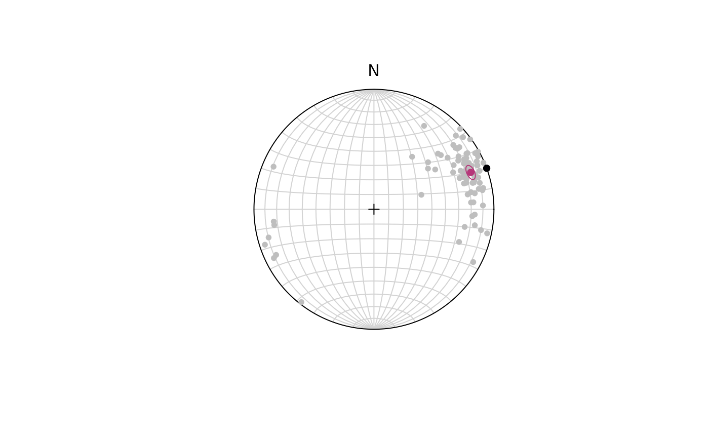
The -value for our hypothesis line:
cenp$pvalue.FUN(line_NULL)
#> [1] 0
With (95% confidence) we rejected the Null Hypothesis that the given line represents the population mean as the p-value is smaller than 5%.
Two-Sample T-Test
Wellner’s Rayleigh-style T-statistic5 measures how different two sets of vectors. The test statistic T is a non-negative measure of dissimilarity between two datasets. The value is zero when the datasets are identical.
wellner(lines, line_NULL)
#> [1] 10.2507
A -value for this test-statistic can be estimated using permutations. The fraction of tests in the computed T-statistic exceeds the observed T for the original data (a number between 0 and 1 inclusive) can be interpreted as a -value for the null hypothesis that the two populations are identical (not merely that their means coincide). Thus, smaller p-values indicate stronger evidence that the two populations differ significantly.
wellner_inference(lines, line_NULL, n_perm = 1000)
#> [1] 0.008
Cluster Vectors
To find k clusters of orientational data, the
sph_cluster() function can be used:
# generate some random vectors:
x1 <- rvmf(100, mu = Ray(90, 0), k = 20)
x2 <- rvmf(100, mu = Ray(0, 0), k = 20)
x3 <- rvmf(100, mu = Ray(0, 90), k = 20)
x123 <- rbind(x1, x2, x3)

# cluster the vectors:
cl <- sph_cluster(x123, k = 3)

# visualize the result:
plot(x123, col = assign_col_d(cl$cluster))

legend_col_d(assign_col_d(unique(cl$cluster)), title = "Cluster")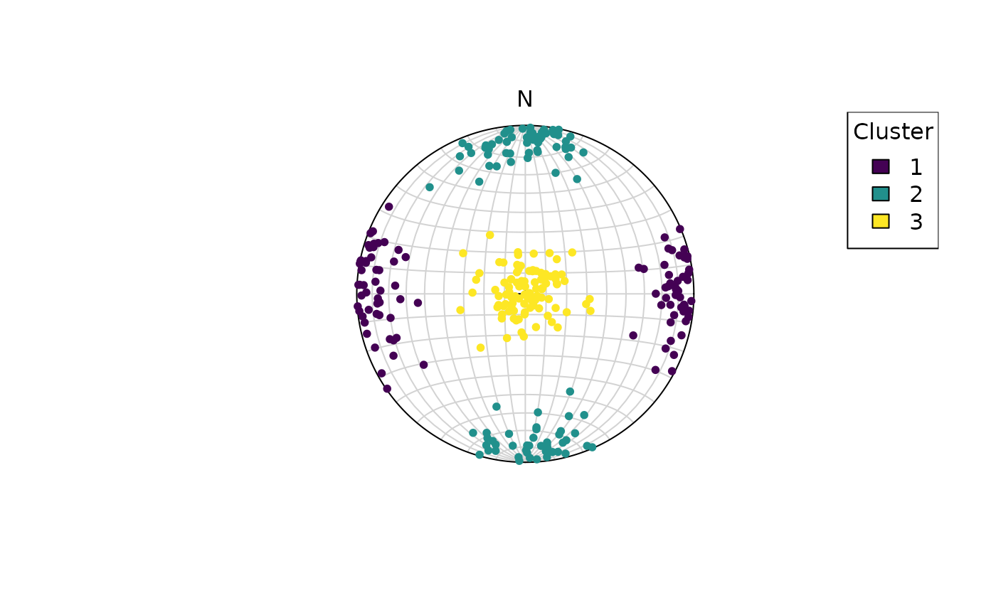
References
Bachmann, F., Hielscher, R., Jupp, P. E., Pantleon, W., Schaeben, H., & Wegert, E. (2010). Inferential statistics of electron backscatter diffraction data from within individual crystalline grains. Journal of Applied Crystallography, 43(6), 1338–1355. https://doi.org/10.1107/S002188981003027X
Davis, J. R., & Titus, S. J. (2017). Modern methods of analysis for three-dimensional orientational data. Journal of Structural Geology, 96, 65–89. https://doi.org/10.1016/j.jsg.2017.01.002
Mardia, K. V., & Jupp, P. E. (2000). Directional Statistics. (K. V. Mardia & P. E. Jupp, Eds.). Hoboken, NJ, USA: Wiley. https://doi.org/10.1002/9780470316979
Scheidegger, A. E. (1964). The tectonic stress and tectonic motion direction in Europe and Western Asia as calculated from earthquake fault plane solutions. Bulletin of the Seismological Society of America, 54(5A), 1519–1528. https://doi.org/10.1785/BSSA05405A1519
Wellner, J. A. (1979) “Permutation Tests for Directional Data.” Ann. Statist. 7(5) 929-943. https://doi.org/10.1214/aos/1176344779