This tutorial introduces the different data types existing in spherical geometry (in particular those used in structural geology).
Data types
Depending on the symmetry of the orientation data, different data types are used to represent orientations in 3D space. The main data types used in structural geology are Rays, Lines, Planes, Pairs, and Faults.
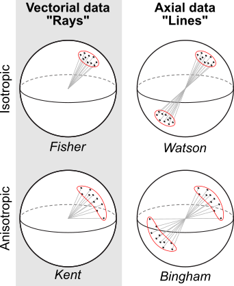
Distinguishing these data types is important each the different symmetries imply different statistical assumption for their distribution. In other words the different data types require different statistical “treatments”.
Don’t worry, once you decided on the symmetry nature of your data, {structr} does the heavy lifting and will (mostly) automatically decide which math operations are appropriate to deal with your data. Below are some more details on the different data types to help you with this important decisions.
Rays (vectorial data)
A Ray is a line with a preferred direction along that
line, i.e. a line with a single start point extending indefinitely in
only one direction (equivalent to a direction in 2D). Examples of
ray-like data include a slip direction, paleomagnetic direction (unless
magnetic reversals are involved), a vorticity vector describing the
sense of slip on a fault, etc.
Ray(120, 30, sense = -1)
#> Ray object (n = 1):
#> azimuth  plunge
#>     300     -30
Lines (axial data)
A Line extends infinitely in both directions (equivalent
to an axis in 2D). Examples of line-like data include a principal stress
directions, strain ellipsoid directions (e.g. stretching lineation),
intersection, fault striae, and crystallographic axes.
Line(120, 30)
#> Line object (n = 1):
#> azimuth  plunge
#>     120      30
Poles to planes
A Plane orientation is described by the normal vector to
a plane. This vector is usually a Line, but can be a
Ray if the younging direction of planes is known. Examples
include the pole to a bedding plane, the pole to a foliation, etc.
Plane(120, 30)
#> Plane object (n = 1):
#> dip_direction           dip
#>           120            30
Pairs and Faults (Plane + Line)
A Pair consists of a Plane and a
Line contained in that plane. Examples are stretching
lineations on a foliation plane.
Pair(120, 30, 75, 15)
#> Pair object (n = 1):
#> dip_direction           dip       azimuth        plunge
#>           120            30            75            15
Fault (Plane + Ray)
A Fault is a special case of a Pair, when the line
component is a Ray object. In other words, a combination of
a plane and a line where the slip direction or sense of motion is
known.
Fault(120, 30, 75, 15, sense = -1)
#> Fault object (n = 1):
#> dip_direction           dip       azimuth        plunge         sense
#>           120            30            75            15            -1
Cartesian coordinates
In general orientation data are expressed in Cartesian Coordinates, that are three-element vectors that represent points or directions in a 3D Cartesian coordinate system given by the direction cosines along the X, Y, and Z axes.
Vec3(1, 0, 0)
#> Vector (Vec3) object (n = 1):
#> x y z
#> 1 0 0
Summary: All data types can be generated using the object creator functions:
Vec3(),Line(),Plane(),Ray(),Pair(), andFault()
Conversions
Any of the spherical objects (Ray, Line, Plane, Pair, Fault) can be
transformed to Cartesian coordinates, or into any other spherical data
type, using the object creator function Vec3(),
Line(), Plane(), Ray(),
Pair(), or Fault() functions. For example:
Line(120, 30) |> Vec3()
#> Vector (Vec3) object (n = 1):
#>          x          y          z
#> -0.4330127  0.7500000  0.5000000
Plane(120, 30) |> Line()
#> Line object (n = 1):
#> azimuth  plunge
#>     300      60

# Combing a plane and a line to a pair:
Pair(Plane(120, 30), Line(120, 30))
#> Pair object (n = 1):
#> dip_direction           dip       azimuth        plunge
#>           120            30           120            30
v <- Pair(Plane(120, 30), Line(120, 30))

Plane(v)
#> Plane object (n = 1):
#> dip_direction           dip
#>           120            30
Line(v)
#> Line object (n = 1):
#> azimuth  plunge
#>     120      30
You can also convert into other data types without transformation,
using as.<data type>() functions. For example,
converting a Line into a Plane:
The functions
as.Vec3(),as.Ray(),as.Line(),as.Plane()as.Pair(), andas.Fault()force a spherical object yo bve coerced into another data type without transformation.
Example
Usually orientation data is stored in a table containing the column dip direction (or strike) and the dip angle of a measured plane…
data(example_planes_df)
head(example_planes_df)
#> # A tibble: 6 × 4
#>   dipdir   dip quality feature_type
#>    <dbl> <dbl>   <dbl> <chr>
#> 1    142    52       3 foliation
#> 2    135    43       3 foliation
#> 3    148    42       3 foliation
#> 4    150    46       3 foliation
#> 5    139    51       3 foliation
#> 6    158    51       3 foliation
or the trend (azimuth) and plunge (inclination) of a measured line…
data(example_lines_df)
head(example_lines_df)
#> # A tibble: 6 × 4
#>   trend plunge quality feature_type
#>   <dbl>  <dbl>   <dbl> <chr>
#> 1    54     13       3 stretching
#> 2    61     15       3 stretching
#> 3    74     14      NA stretching
#> 4    80     19      NA stretching
#> 5    63     17      NA stretching
#> 6    76     10      NA stretching
To convert these data frames to spherical objects, use the
Plane() and Line() functions from the
structr package. These functions take the dip direction and
dip angle for planes, and the trend and plunge for lines as
arguments.
data(example_planes)
planes <- Plane(example_planes_df$dipdir, example_planes_df$dip)
lines <- Line(example_lines_df$trend, example_lines_df$plunge)
If the raw data was imported using
read_strabo_JSON()this step is not necessary as the data will come already in the correct format.
The spherical objects can be easily converted into Cartesian
coordinate vectors using the function Vec3():
lines_vector <- Vec3(lines)
head(lines_vector)
#> Vector (Vec3) object (n = 6):
#>              x         y         z
#> [1,] 0.5727204 0.7882819 0.2249511
#> [2,] 0.4682901 0.8448178 0.2588190
#> [3,] 0.2674497 0.9327081 0.2419219
#> [4,] 0.1641876 0.9311540 0.3255682
#> [5,] 0.4341533 0.8520738 0.2923717
#> [6,] 0.2382466 0.9555548 0.1736482
Convert a Plane’s pole to a Line: