Skip to contents

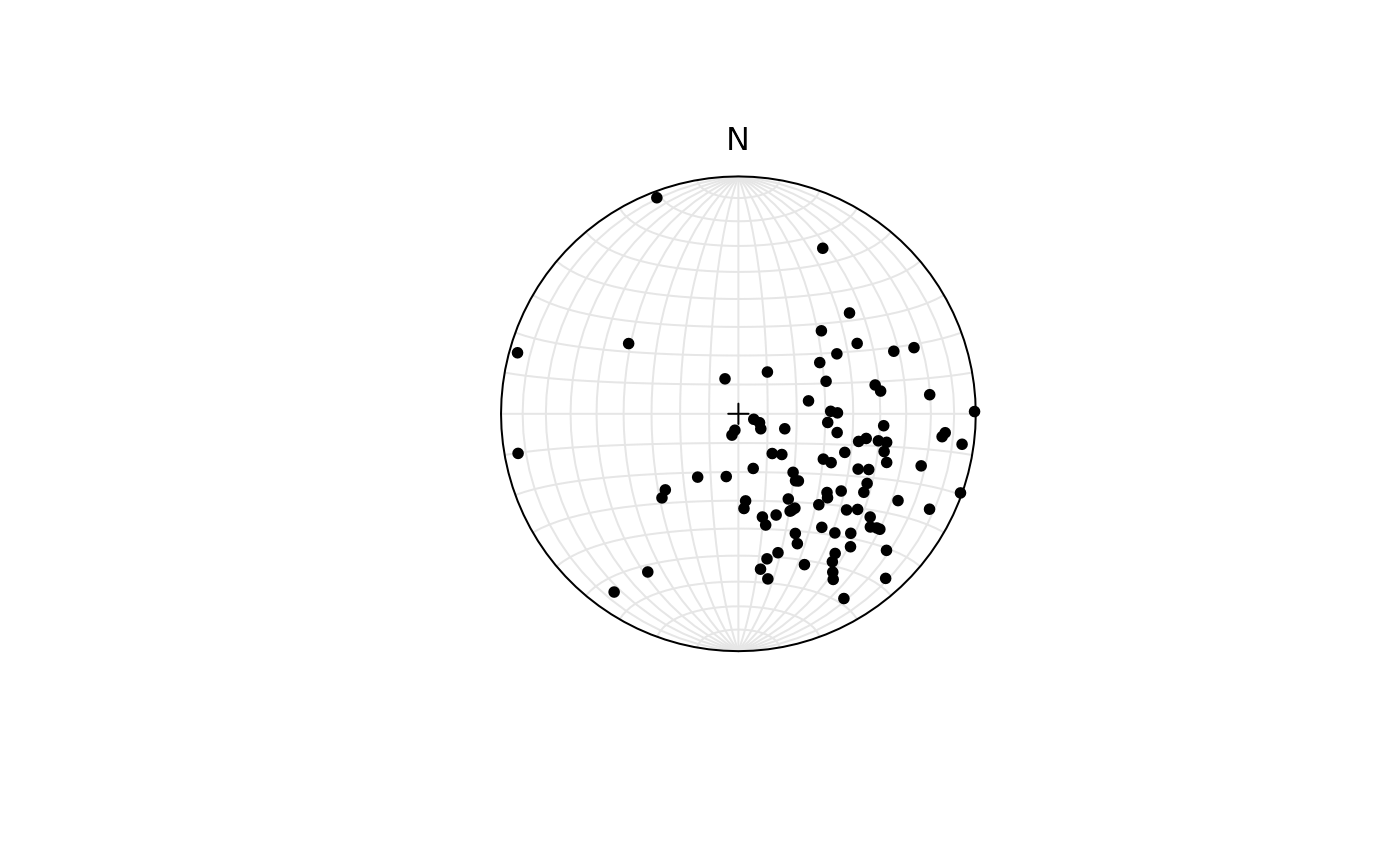
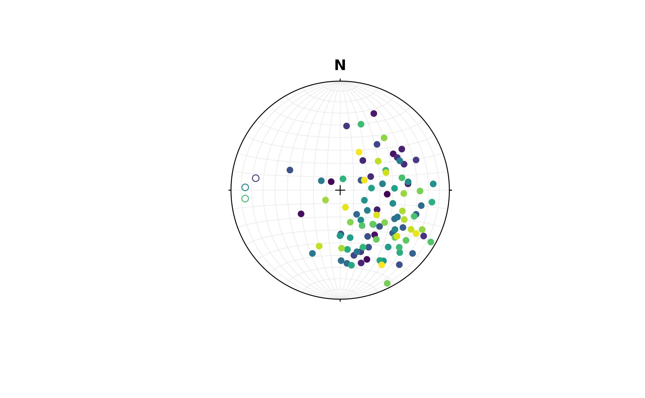
Density and random generation for the spherical normal distribution with mean and kappa.

Usage

rvmf(n = 100, mu = Vec3(1, 0, 0), k = 5)

dvmf(x, mu, k = 5)

Source

Adapted fom rotasym::r_vMF() and rotasym::d_vMF()

Arguments

n

integer. number of random samples to be generated

k

numeric. The concentration parameter (\(\kappa\)) of the the von Mises-Fisher distribution

x, mu

object of class "Vec3", "Line" or "Plane"

See also

runif.spherical() for alternative algorithms to generate uniform distributed samples on a sphere, rkent() for Kent distribution, rfb() for Fisher-Bingham distribution.

Examples

set.seed(20250411)
x <- rvmf(100, mu = Line(120, 50), k = 5)
dvmf(x, mu = Line(120, 50))
#>                [,1]
#>   [1,] 0.3539638684
#>   [2,] 0.3456838512
#>   [3,] 0.3298219243
#>   [4,] 0.2878725467
#>   [5,] 0.3416723702
#>   [6,] 0.3087497280
#>   [7,] 0.5029607511
#>   [8,] 0.6655797562
#>   [9,] 0.7907738489
#>  [10,] 0.0037954383
#>  [11,] 0.6941862756
#>  [12,] 0.2215063746
#>  [13,] 0.6595268453
#>  [14,] 0.0005060201
#>  [15,] 0.7195109535
#>  [16,] 0.0733917426
#>  [17,] 0.6958226791
#>  [18,] 0.6722856633
#>  [19,] 0.6780233707
#>  [20,] 0.3776313507
#>  [21,] 0.6946564573
#>  [22,] 0.5766307194
#>  [23,] 0.7759395592
#>  [24,] 0.7901589106
#>  [25,] 0.6272959464
#>  [26,] 0.4489849106
#>  [27,] 0.6963171147
#>  [28,] 0.2077329205
#>  [29,] 0.4884814860
#>  [30,] 0.3942015612
#>  [31,] 0.7024778981
#>  [32,] 0.0009551707
#>  [33,] 0.7484831155
#>  [34,] 0.6860774055
#>  [35,] 0.0991952887
#>  [36,] 0.5446196691
#>  [37,] 0.2645460130
#>  [38,] 0.4137899293
#>  [39,] 0.2787976931
#>  [40,] 0.0008812961
#>  [41,] 0.3279258107
#>  [42,] 0.0575149554
#>  [43,] 0.3095756565
#>  [44,] 0.6331699361
#>  [45,] 0.5687413756
#>  [46,] 0.3877695235
#>  [47,] 0.7037452677
#>  [48,] 0.6272525066
#>  [49,] 0.4839627489
#>  [50,] 0.0074576675
#>  [51,] 0.0703558313
#>  [52,] 0.2590478470
#>  [53,] 0.1393608634
#>  [54,] 0.6407961152
#>  [55,] 0.1680944634
#>  [56,] 0.1146974769
#>  [57,] 0.6714866658
#>  [58,] 0.3713923453
#>  [59,] 0.3256224108
#>  [60,] 0.2225528050
#>  [61,] 0.7945046115
#>  [62,] 0.0302259400
#>  [63,] 0.7334812584
#>  [64,] 0.7544944369
#>  [65,] 0.6794339163
#>  [66,] 0.7217814257
#>  [67,] 0.0848180617
#>  [68,] 0.7887117130
#>  [69,] 0.0003715124
#>  [70,] 0.3587100009
#>  [71,] 0.4406101476
#>  [72,] 0.1213333354
#>  [73,] 0.6950889621
#>  [74,] 0.4436411860
#>  [75,] 0.5731018054
#>  [76,] 0.1131717267
#>  [77,] 0.3333639706
#>  [78,] 0.4203673749
#>  [79,] 0.7774430701
#>  [80,] 0.3796139755
#>  [81,] 0.2822486781
#>  [82,] 0.1697738070
#>  [83,] 0.1937737433
#>  [84,] 0.7613930727
#>  [85,] 0.6273298854
#>  [86,] 0.2486908813
#>  [87,] 0.4865129857
#>  [88,] 0.6431243513
#>  [89,] 0.5875447305
#>  [90,] 0.3346200855
#>  [91,] 0.5347723283
#>  [92,] 0.0008189982
#>  [93,] 0.4533583635
#>  [94,] 0.4058711922
#>  [95,] 0.4600893515
#>  [96,] 0.4565435898
#>  [97,] 0.6740864570
#>  [98,] 0.1553085088
#>  [99,] 0.2685622708
#> [100,] 0.4133662866
plot(x)