3D strain diagram using the Hsu (1965) method to display the amount of the natural octahedral strain, \(\bar{\epsilon}_s\) (Nádai, 1950) and Lode's parameter for the symmetry of strain \(\nu\) (Lode, 1926).
Usage
hsu_plot(x, ...)

# S3 method for class 'ortensor'
hsu_plot(
  x,
  labels = NULL,
  add = FALSE,
  es.max = 3,
  main = "Hsu diagram",
  weights = NULL,
  ...
)

# S3 method for class 'spherical'
hsu_plot(x, weights = NULL, ...)

# S3 method for class 'ellispoid'
hsu_plot(x, ...)

# Default S3 method
hsu_plot(
  x,
  labels = NULL,
  add = FALSE,
  es.max = 3,
  main = "Hsu diagram",
  guides = NULL,
  ...
)

# S3 method for class 'list'
hsu_plot(x, labels = NULL, add = FALSE, es.max = 3, main = "Hsu diagram", ...)
Arguments
- x
accepts the following objects: a two-column matrix where first column is the ratio of maximum strain and intermediate strain (X/Y) and second column is the the ratio of intermediate strain and minimum strain (Y/Z); objects of class
"Vec3","Line","Ray","Plane","ortensor"and"ellipsoid"objects. Tensor objects can also be lists of such objects ("ortensor"and"ellipsoid").- ...
plotting arguments passed to
graphics::points()- labels
character. text labels
- add
logical. Should data be plotted to an existing plot?
- es.max
maximum strain for scaling.
- main
character. The main title (on top).
- weights
numeric. Weightings
- guides
logical. Whether guides should be added to the plot. Defaults to
getOption("structr.guides").
Details
The amount of strain related to the natural octahedral unit shear \(\bar{\gamma}_o\) is (Nádai, 1963, p.73): $$\bar{\epsilon}_s = \frac{\sqrt{3}}{2} \bar{\gamma}_o$$ where \(\bar{\gamma}_o\) is defined as $$\bar{\gamma}_o = \frac{2}{3} \sqrt{(\bar{\epsilon}_1 - \bar{\epsilon}_2)^2 + (\bar{\epsilon}_2 - \bar{\epsilon}_3)^2 + (\bar{\epsilon}_3 - \bar{\epsilon}_1)^2}$$ and \(\bar{\epsilon}\) is the natural strain (\(\bar{\epsilon} = \log{1+\epsilon}\)) and \(\epsilon\) is the conventional strain given by \(\epsilon = \frac{l-l_0}{l_0}\) where \(l\) and \(l_0\) is the length after and before the strain, respectively (Nádai, 1959, p.70). The amount of strain \(\bar{\epsilon}_s\) is directly proportional to the amount of mechanical work applied in the coaxial component of strain.
The symmetry of strain is defined by Lode’s (1926, p.932) ratio (\(\nu\)): $$\nu = \frac{2 \bar{\epsilon}_2 - \bar{\epsilon}_1 - \bar{\epsilon}_3}{\bar{\epsilon}_1 - \bar{\epsilon}_3}$$ The values range between -1 and +1, where -1 gives constriction, 0 gives plane strain, and +1 gives flattening.
Note
Hossack (1968) was the first one to use this graphical representation of 3D strain and called the plot "Strain plane plot"
References
Lode, W. (1926). Versuche über den Einfluß der mittleren Hauptspannung auf das Fließen der Metalle Eisen. Kupfer und Nickel. Zeitschrift Für Physik, 36(11–12), 913–939. doi:10.1007/BF01400222
Nádai, A. (1950). Theory of flow and fracture of solids. McGraw-Hill.
Hsu, T. C. (1966). The characteristics of coaxial and non-coaxial strain paths. Journal of Strain Analysis, 1(3), 216–222. doi:10.1243/03093247V013216
Hossack, J. R. (1968). Pebble deformation and thrusting in the Bygdin area (Southern Norway). Tectonophysics, 5(4), 315–339. doi:10.1016/0040-1951(68)90035-8
See also
lode() for Lode parameter, and nadai for natural octahedral strain.
ellipsoid() class, ortensor() class
Other fabric-plot:
flinn_plot(),
vollmer-plot,
woodcock_plot()
Examples
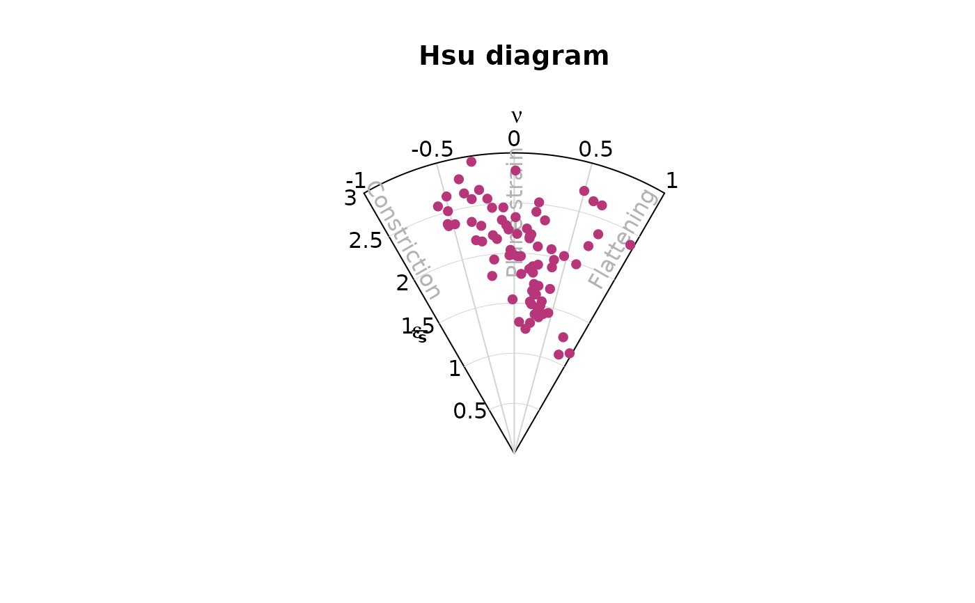
# default
R_XY <- holst[, "R_XY"]
R_YZ <- holst[, "R_YZ"]
hsu_plot(cbind(R_XY, R_YZ), col = "#B63679", pch = 16, type = "b")
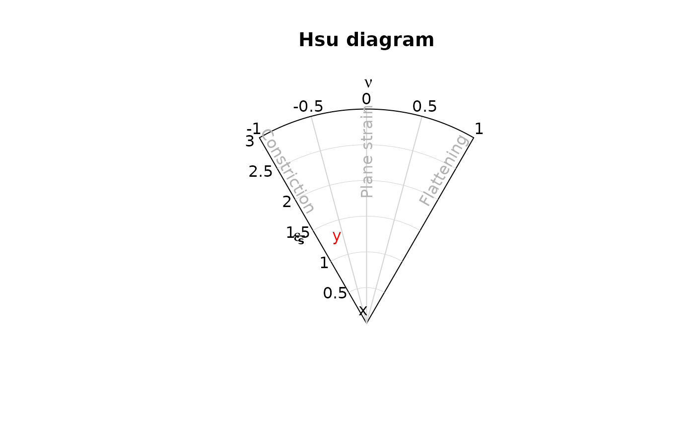
 # orientation data
set.seed(20250411)
mu <- Line(120, 50)
x <- rvmf(100, mu = mu, k = 1)
hsu_plot(x, labels = "x")
set.seed(20250411)
y <- rvmf(100, mu = mu, k = 20)
hsu_plot(ortensor(y), labels = "y", col = "red", add = TRUE)
# orientation data
set.seed(20250411)
mu <- Line(120, 50)
x <- rvmf(100, mu = mu, k = 1)
hsu_plot(x, labels = "x")
set.seed(20250411)
y <- rvmf(100, mu = mu, k = 20)
hsu_plot(ortensor(y), labels = "y", col = "red", add = TRUE)
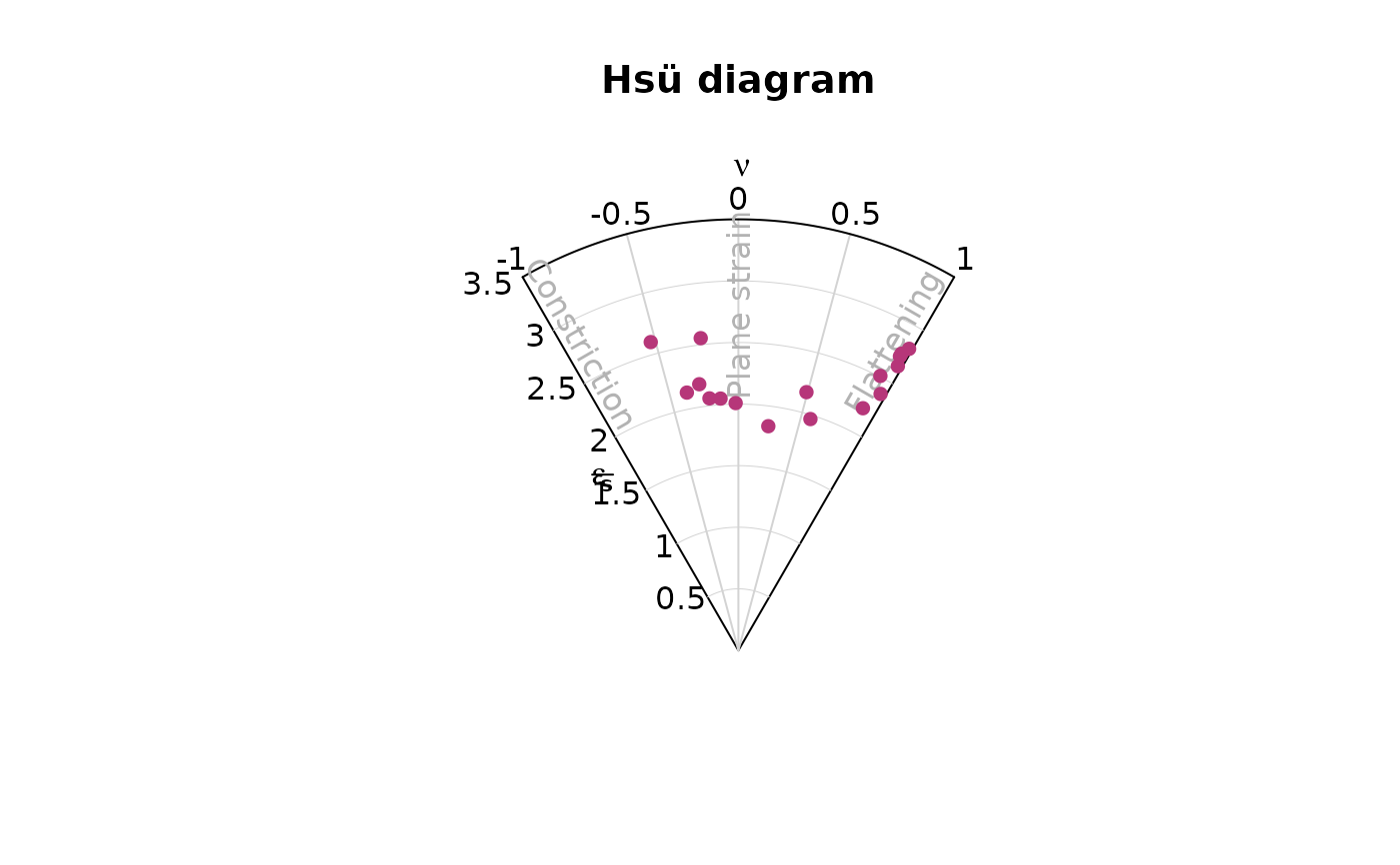
 # ellipsoid objects
hossack_ell <- lapply(seq.int(nrow(hossack1968)), function(i) {
ellipsoid_from_stretch(hossack1968[i, 3], hossack1968[i, 2], hossack1968[i, 1])
})
hsu_plot(hossack_ell, col = "#B63679", pch = 16)
# ellipsoid objects
hossack_ell <- lapply(seq.int(nrow(hossack1968)), function(i) {
ellipsoid_from_stretch(hossack1968[i, 3], hossack1968[i, 2], hossack1968[i, 1])
})
hsu_plot(hossack_ell, col = "#B63679", pch = 16)