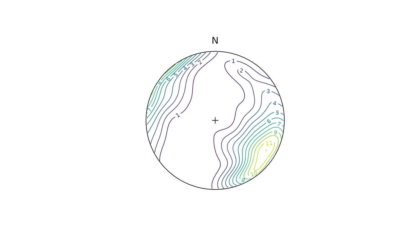
Kamb counts and densities on the sphere. contour plots the contour lines,
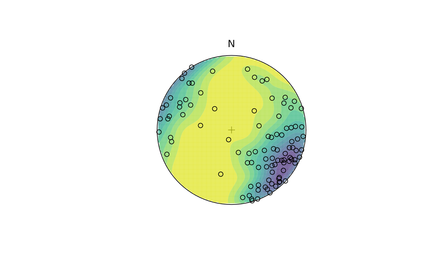
contourf displays a contour plot with the areas between the contours filled,
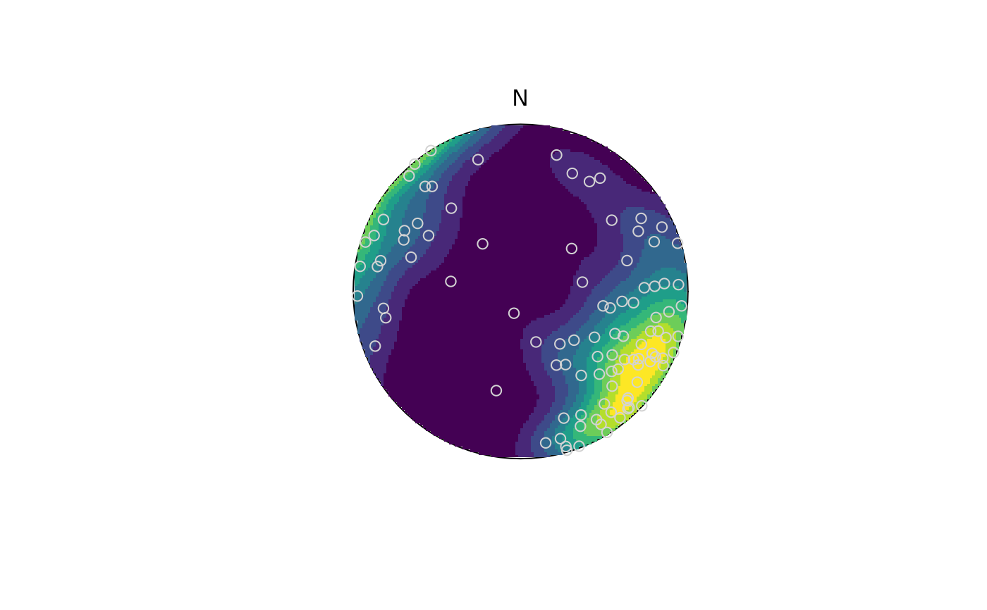
and image creates a dense grid of colored rectangles.
Usage
# S3 method for class 'spherical'
contour(
  x,
  add = FALSE,
  nlevels = 10L,
  density.params = list(),
  col.palette = viridis::viridis,
  col = NULL,
  col.params = list(),
  upper.hem = NULL,
  radius = NULL,
  ...
)

# S3 method for class 'sph_density'
contour(
  x,
  add = FALSE,
  nlevels = 10L,
  density.params = list(),
  col.palette = viridis::viridis,
  col = NULL,
  col.params = list(),
  upper.hem = NULL,
  radius = NULL,
  ...
)

contourf(
  x,
  add = FALSE,
  nlevels = 10L,
  density.params = list(),
  col.palette = viridis::viridis,
  col.params = list(),
  upper.hem = NULL,
  radius = NULL,
  ...
)

# S3 method for class 'spherical'
image(
  x,
  add = FALSE,
  nlevels = 10L,
  density.params = list(),
  col.palette = viridis::viridis,
  col.params = list(),
  upper.hem = NULL,
  radius = NULL,
  ...
)

# S3 method for class 'sph_density'
image(
  x,
  add = FALSE,
  nlevels = 10L,
  density.params = list(),
  col.palette = viridis::viridis,
  col.params = list(),
  upper.hem = NULL,
  radius = NULL,
  ...
)
Arguments
- x
object of class
"Vec3","Line","Ray","Plane"or'sph_density'(for plotting only).- add
logical. Whether the contours should be added to an existing plot.
- nlevels
integer. Number of contour levels for plotting
- density.params
list. Optional arguments passed to
density.spherical(), such asFUN,n,sigma, andweights- col.palette
a color palette function to be used to assign colors in the plot.
- col
colour(s) for the contour lines drawn. If
NULL, lines are color based oncol.palette.- col.params
list. Arguments passed to
col.palette- upper.hem
logical. Whether the projection is shown for upper hemisphere (
TRUE) or lower hemisphere (FALSE). Defaults togetOption("structr.upper.hem").- radius
numeric. Radius of circle. Defaults to
getOption("structr.radius").- ...
optional parameters passed to
graphics::image()orgraphics::contour().
See also
Other stereo-plot:
arrows,
fault-plot,
lines,
plot-spherical,
points.spherical(),
stereo_cones,
stereo_confidence(),
stereo_lines(),
stereo_point(),
stereo_segment(),
stereoplot(),
stereoplot_guides(),
stereoplot_ticks(),
text.spherical()
Other density:
density,
density-funs
Examples
set.seed(20250411)
x <- rfb(100, mu = Line(120, 10), k = 5, A = diag(c(-1, 0, 1)))
contour(x)
 x_density <- density(x)
contourf(x_density,
col.params = list(direction = -1, begin = .05, end = .95, alpha = .75)
)
stereo_point(x, col = "black", pch = 21)
x_density <- density(x)
contourf(x_density,
col.params = list(direction = -1, begin = .05, end = .95, alpha = .75)
)
stereo_point(x, col = "black", pch = 21)
 image(x)
stereo_point(x, col = "lightgrey", pch = 21)
image(x)
stereo_point(x, col = "lightgrey", pch = 21)
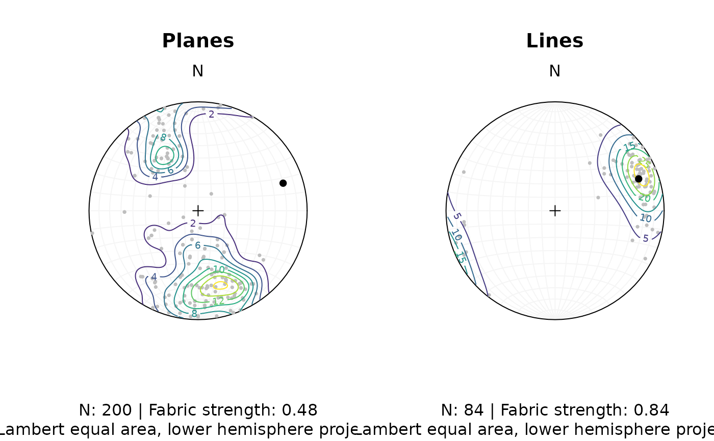
 # complete example:
par(mfrow = c(1, 2))
wp <- 6 / ifelse(is.na(example_planes_df$quality), 6, example_planes_df$quality)
my_planes <- Plane(example_planes_df$dipdir, example_planes_df$dip)
fabric_p <- vollmer(my_planes)["D"]
my_planes_eig <- ot_eigen(my_planes)
stereoplot(guides = TRUE, col = "grey96")
points(my_planes, col = "grey", pch = 16, cex = .5)
contour(my_planes, add = TRUE, weights = wp)
points(my_planes_eig$vectors[3, ], col = "black", pch = 16)
lines(my_planes_eig$vectors[3, ], ang = 90, col = "black", pch = 16)
title(
main = "Planes",
sub = paste0(
"N: ", nrow(my_planes), " | Fabric strength: ", round(fabric_p, 2),
"\nLambert equal area, lower hemisphere projection"
)
)
my_lines <- Line(example_lines_df$trend, example_lines_df$plunge)
wl <- 6 / ifelse(is.na(example_lines_df$quality), 6, example_lines_df$quality)
fabric_l <- vollmer(my_lines)["D"]
stereoplot(guides = TRUE, col = "grey96")
points(my_lines, col = "grey", pch = 16, cex = .5)
contour(my_lines, add = TRUE, weights = wl)
points(sph_mean(my_lines, w = wl), col = "black", pch = 16)
title(
main = "Lines",
sub = paste0(
"N: ", nrow(my_lines), " | Fabric strength: ", round(fabric_l, 2),
"\nLambert equal area, lower hemisphere projection"
)
)
# complete example:
par(mfrow = c(1, 2))
wp <- 6 / ifelse(is.na(example_planes_df$quality), 6, example_planes_df$quality)
my_planes <- Plane(example_planes_df$dipdir, example_planes_df$dip)
fabric_p <- vollmer(my_planes)["D"]
my_planes_eig <- ot_eigen(my_planes)
stereoplot(guides = TRUE, col = "grey96")
points(my_planes, col = "grey", pch = 16, cex = .5)
contour(my_planes, add = TRUE, weights = wp)
points(my_planes_eig$vectors[3, ], col = "black", pch = 16)
lines(my_planes_eig$vectors[3, ], ang = 90, col = "black", pch = 16)
title(
main = "Planes",
sub = paste0(
"N: ", nrow(my_planes), " | Fabric strength: ", round(fabric_p, 2),
"\nLambert equal area, lower hemisphere projection"
)
)
my_lines <- Line(example_lines_df$trend, example_lines_df$plunge)
wl <- 6 / ifelse(is.na(example_lines_df$quality), 6, example_lines_df$quality)
fabric_l <- vollmer(my_lines)["D"]
stereoplot(guides = TRUE, col = "grey96")
points(my_lines, col = "grey", pch = 16, cex = .5)
contour(my_lines, add = TRUE, weights = wl)
points(sph_mean(my_lines, w = wl), col = "black", pch = 16)
title(
main = "Lines",
sub = paste0(
"N: ", nrow(my_lines), " | Fabric strength: ", round(fabric_l, 2),
"\nLambert equal area, lower hemisphere projection"
)
)