Visualization of small-circles and great-circles in a stereographic or equal-area projection.
Arguments
- x
object of class
"Vec3","Line","Ray","Plane","Pair", or"Fault", where the rows are the observations and the columns are the coordinates.- d
numeric. conical angle in degrees.
- col, lty, lwd
color, line type, and line width parameters
- N
integer. number of points to calculate
- upper.hem
logical. Whether the projection is shown for upper hemisphere (
TRUE) or lower hemisphere (FALSE). Defaults togetOption("structr.upper.hem").- earea
logical. Projection, either
TRUEfor Lambert equal-area projection, orFALSEfor meridional stereographic projection. Defaults togetOption("structr.earea").- fill
logical. Whether to fill the inner part of the small-circle?
FALSEby default.- border
Color of the filled small-circle's outline (ignored if
fill=FALSE)- radius
numeric. Radius of circle. Defaults to
getOption("structr.radius").- ...
optional graphical parameters passed to
graphics::lines()and (iffill=TRUE)graphics::polygon()
Examples
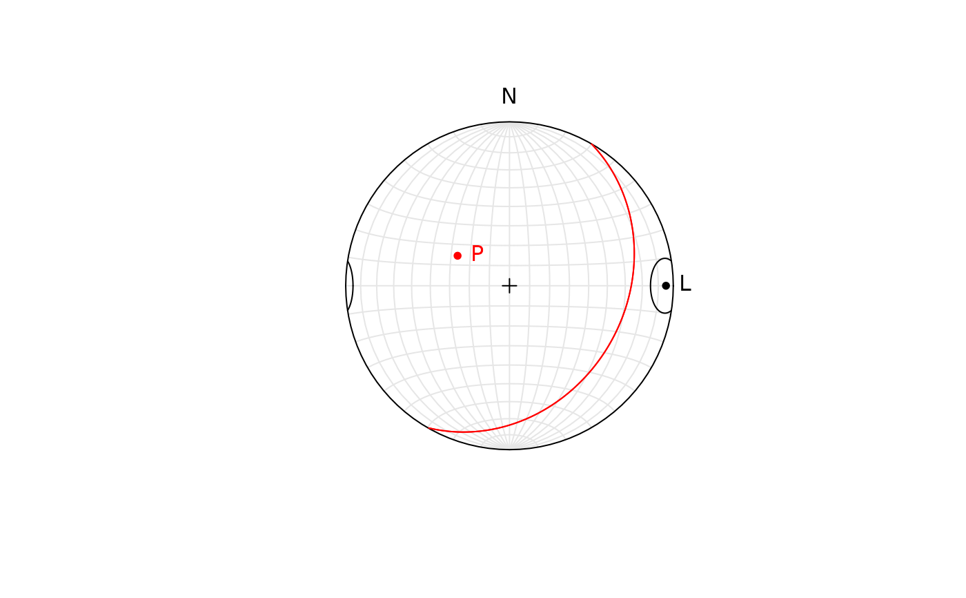
stereoplot()
stereo_point(Line(90, 5), lab = "L")
stereo_smallcircle(Line(90, 5), d = 10)
stereo_point(Plane(120, 30), lab = "P", col = "red")
stereo_greatcircle(Plane(120, 30), col = "red")
 stereoplot()
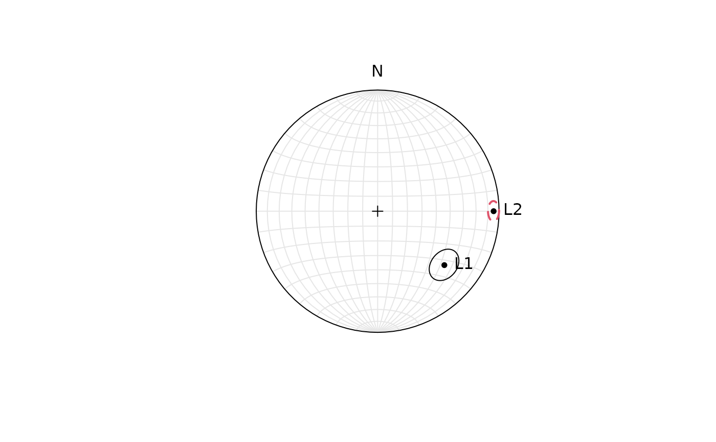
stereo_point(Line(c(129, 90), c(30, 5)), lab = c("L1", "L2"))
stereo_smallcircle(Line(c(129, 90), c(30, 5)), d = c(10, 5),
col = 1:2, lty = 1:2, lwd = 1:2)
stereoplot()
stereo_point(Line(c(129, 90), c(30, 5)), lab = c("L1", "L2"))
stereo_smallcircle(Line(c(129, 90), c(30, 5)), d = c(10, 5),
col = 1:2, lty = 1:2, lwd = 1:2)
 #> [[1]]
#> NULL
#>
#> [[2]]
#> NULL
#>
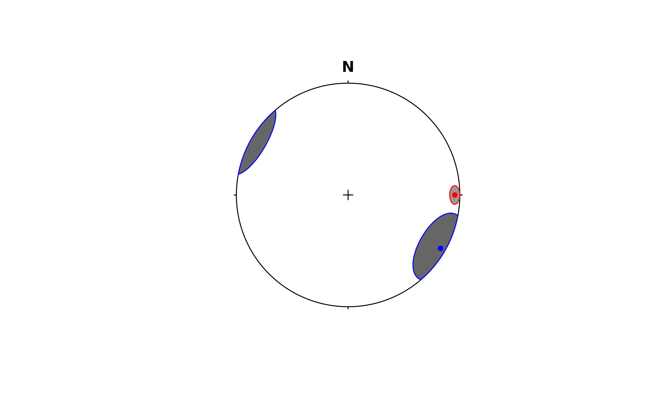
# Filled cones:
stereoplot()
stereo_smallcircle(Line(c(90, 120), c(5, 5)), d = c(5, 20),
col = c('grey60', 'grey40'), border = c('red', 'blue'), fill = TRUE)
stereo_point(Line(c(90, 120), c(5, 5)), col = c('red', 'blue'))
#> [[1]]
#> NULL
#>
#> [[2]]
#> NULL
#>
# Filled cones:
stereoplot()
stereo_smallcircle(Line(c(90, 120), c(5, 5)), d = c(5, 20),
col = c('grey60', 'grey40'), border = c('red', 'blue'), fill = TRUE)
stereo_point(Line(c(90, 120), c(5, 5)), col = c('red', 'blue'))