Add fault data to existing plot

Add fault data to existing plot

Usage

fault_plot(x, type = c("angelier", "hoeppener"), ...)

hoeppener(x, pch = 1, col = "black", cex = 1, bg = NULL, points = TRUE, ...)

angelier(
  x,
  pch = 1,
  lwd = 1,
  lty = 1,
  col = "black",
  cex = 1,
  points = TRUE,
  bg = NULL,
  ...
)

Arguments

x

"Fault" object where the rows are the observations, and the columns the coordinates.

type

character. One of "angelier" (for "Angelier plot") or "hoeppener" (for "Hoeppener plot"). See details.

...

arguments passed to stereo_arrows()

points

logical. Whether the lineation points (Angelier plot) or poles (Hoeppener plot) should be added to the plot

lty, lwd, cex, pch, col, bg

plotting parameters

Details

Angelier plot shows all planes as great circles and lineations as points. Fault striae are plotted as vectors on top of the lineation pointing in the movement direction of the hangingwall. Easy to read in case of homogeneous or small datasets.

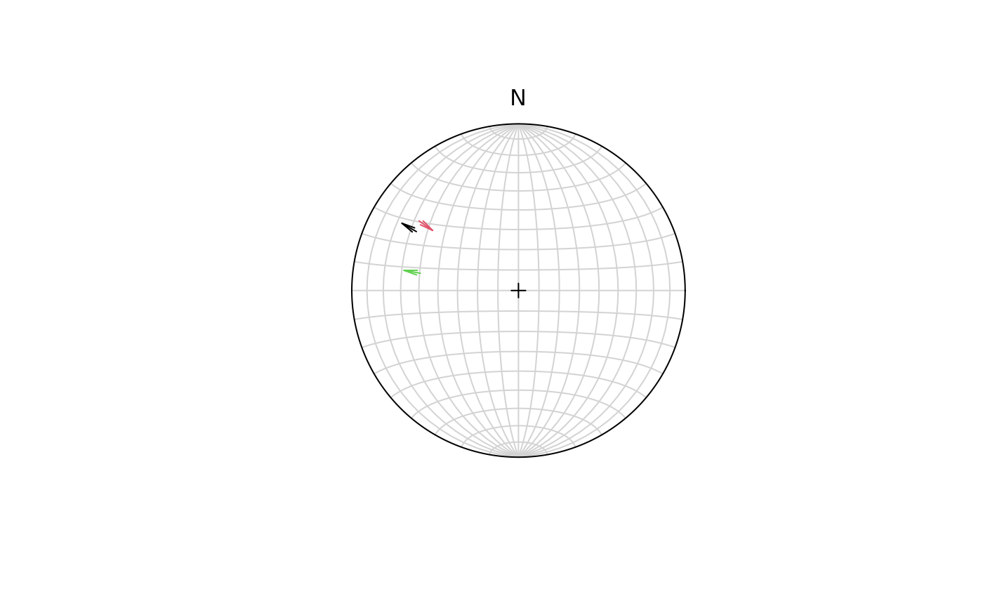
Hoeppener plot shows all planes as poles while lineations are not shown. Fault striae are plotted as vectors on top of poles pointing in the movement direction of the hangingwall. Useful in case of large or heterogeneous datasets.

References

Angelier, J. Tectonic analysis of fault slip data sets, J. Geophys. Res. 89 (B7), 5835-5848 (1984)

Hoeppener, R. Tektonik im Schiefergebirge. Geol Rundsch 44, 26-58 (1955). https://doi.org/10.1007/BF01802903

See also

stereo_arrows()

Examples

f <- Fault(
  c("a" = 120, "b" = 125, "c" = 100),
  c(60, 62, 50),
  c(110, 25, 30),
  c(58, 9, 23),
  c(1, -1, 1)
)

stereoplot(title = "Angelier plot")
angelier(f, col = 1:nrow(f), pch = 16, scale = 0.1)


stereoplot(title = "Hoeppener plot")
hoeppener(f, col = 1:nrow(f), cex = 1, scale = 0.1, points = FALSE)


# or
stereoplot()
fault_plot(f, type = "hoeppener", col = 1:nrow(f), cex = 1, scale = 0.1, points = FALSE)