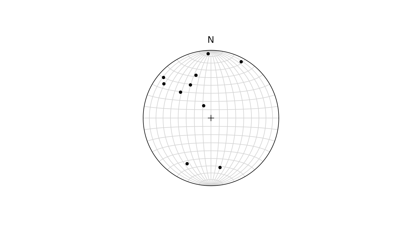
Plot spherical objects

Usage

# S3 method for class 'Line'
plot(x, upper.hem = FALSE, earea = TRUE, grid.params = list(), ...)

# S3 method for class 'Vec3'
plot(x, upper.hem = FALSE, earea = TRUE, grid.params = list(), ...)

# S3 method for class 'Ray'
plot(x, upper.hem = FALSE, earea = TRUE, grid.params = list(), ...)

# S3 method for class 'Plane'
plot(x, upper.hem = FALSE, earea = TRUE, grid.params = list(), ...)

# S3 method for class 'Pair'
plot(x, upper.hem = FALSE, earea = TRUE, grid.params = list(), ...)

# S3 method for class 'Fault'
plot(x, upper.hem = FALSE, earea = TRUE, grid.params = list(), ...)

Arguments

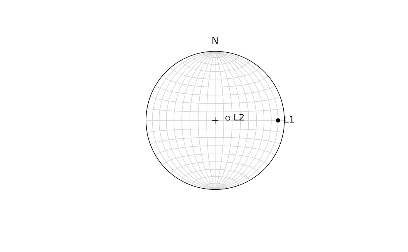
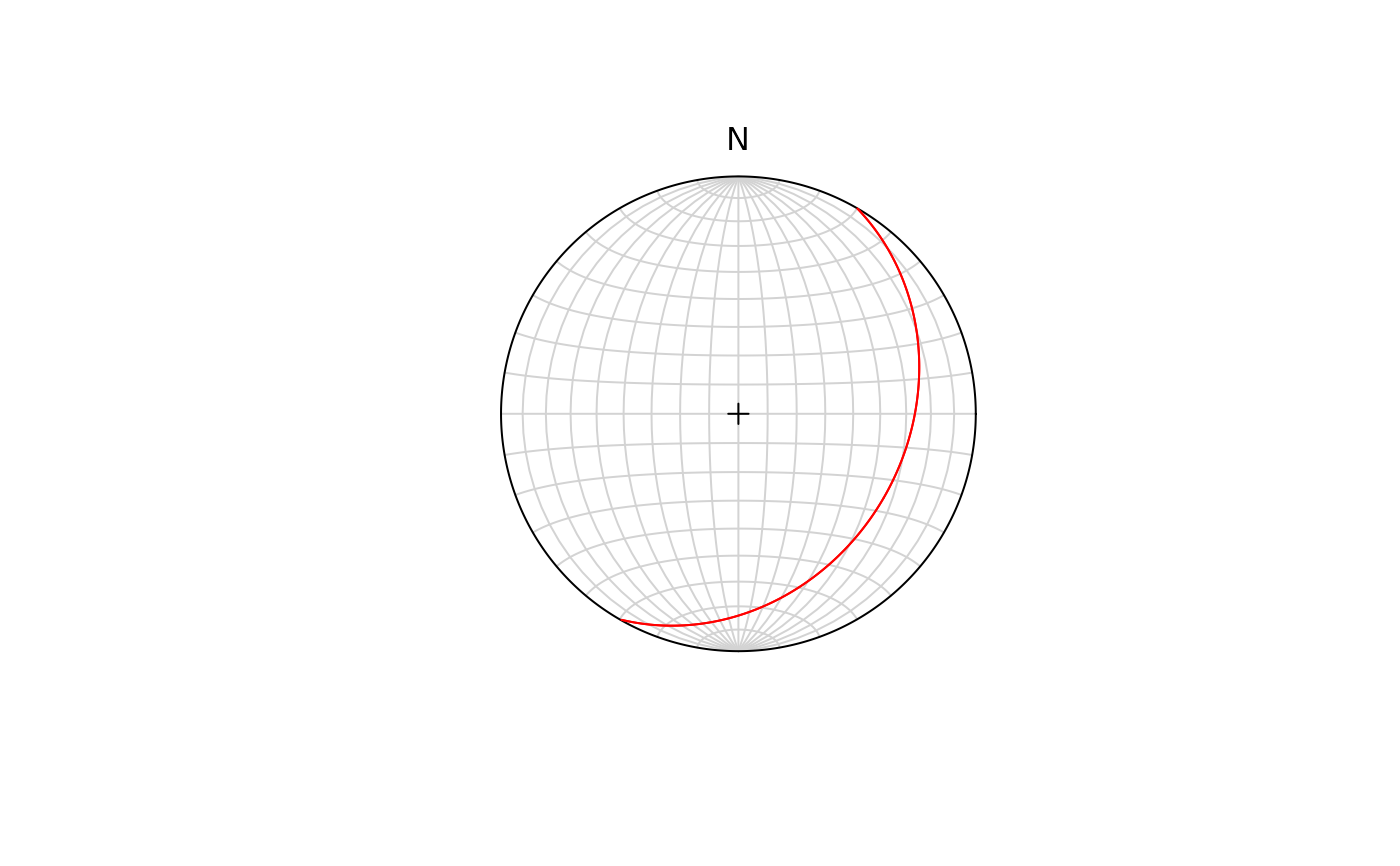
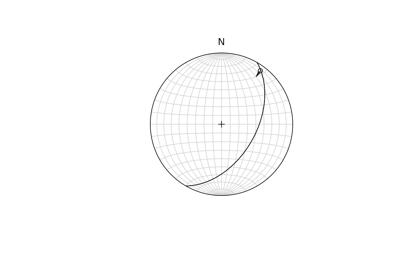
x: object of class "Vec3", "Line", "Ray", "Plane", "Pair", or "Fault", where the rows are the observations and the columns are the coordinates.
upper.hem: logical. Whether the projection is shown for upper hemisphere (TRUE) or lower hemisphere (FALSE, the default).
earea: logical TRUE for Lambert equal-area projection (also "Schmidt net"; the default), or FALSE for meridional stereographic projection (also "Wulff net" or "Stereonet").
grid.params: list.
...: parameters passed to stereo_point(), stereo_smallcircle(), stereo_greatcircle(), or fault_plot()

Details

If x is a Ray, than solid symbols show rays pointing in the lower hemisphere, and open symbols point into the upper hemisphere

Examples

plot(rvmf(10, mu = Vec3(1, 0, 0))) # Vec

plot(Line(c(90, 80), c(10, 75)), lab = c("L1", "L2"))

plot(Ray(c(90, 80), c(10, 75), sense = c(1, -1)), lab = c("L1", "L2"))

plot(Plane(120, 30), col = "red")

plot(Pair(120, 50, 36, 8))

plot(Fault(120, 50, 36, 8, -1))