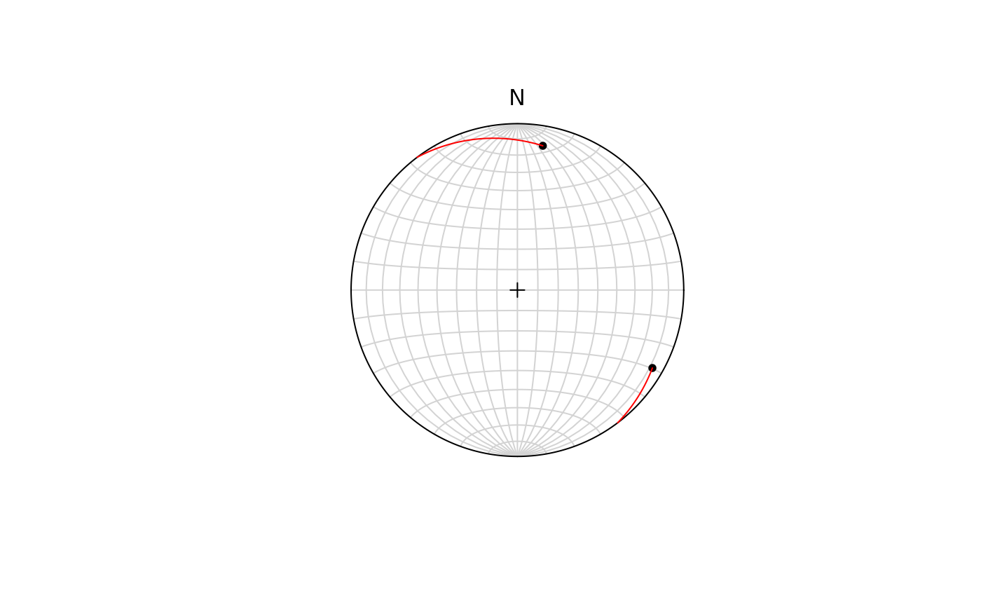
Plots the great-circle segment between two vectors
Arguments
- x, y
objects of class
"Vec3","Line","Ray", or"Plane"- upper.hem
logical. Whether the projection is shown for upper hemisphere (
TRUE) or lower hemisphere (FALSE, the default).- earea
logical
TRUEfor Lambert equal-area projection (also "Schmidt net"; the default), orFALSEfor meridional stereographic projection (also "Wulff net" or "Stereonet").- n
integer. number of points along great-circle (100 by default)
- BALL.radius
numeric size of sphere
- ...
optional graphical parameters passed to
graphics::lines()
Examples
x <- Line(120, 7)
y <- Line(10, 13)
plot(rbind(x, y))
stereo_segment(x, y, col = "red")
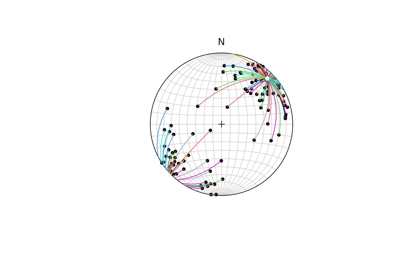
 # For multiple segments use lapply():
set.seed(20250411)
mu <- Line(45, 10)
x <- rvmf(100, mu = mu) |> Line()
plot(x)
invisible(lapply(seq_len(nrow(x)), FUN = function(i) {
stereo_segment(x[i, ], mu, col = i)
}))
points(mu, pch = 16, col = "white")
# For multiple segments use lapply():
set.seed(20250411)
mu <- Line(45, 10)
x <- rvmf(100, mu = mu) |> Line()
plot(x)
invisible(lapply(seq_len(nrow(x)), FUN = function(i) {
stereo_segment(x[i, ], mu, col = i)
}))
points(mu, pch = 16, col = "white")