Stress Inversion for Fault-Slip Data after Michael (1984)
Source:R/stress_inversion.R
slip_inversion_michael.RdDirect stress inversion (based on Michael, 1984) determines the orientation of the principal stresses from fault slip data. Confidence intervals are estimated by bootstrapping. This inversion is simplified by the assumption that the magnitude of the tangential traction on the various fault planes, at the time of rupture, is similar.
Arguments
- x
"Fault"object where the rows are the observations, and the columns the coordinates. Object must be complete, i.e. noNAvalues. For Michael's, Angelier's, and Yamaji-Sato's methods, at least 4 rows of fault measurements are required, while Hansen's method requires at least 7.- n_iter
integer. Number of bootstrap replicates (100 by default)
- conf.level
numeric. Confidence level of the interval (0.95 by default)
- flip
logical. Flip if you want to have the negative stress tensor, i.e. sigma 1 and 3 will be flipped.
- ...
optional parameters passed to
confidence_ellipse()
Value
Additionally, this child functions appends the following list components:
principal_axes_CIlist containing the confidesnce ellipses for the 3 principal stress vectors. See
confidence_ellipse()for details.principal_vals_CI3-column vector containing the lower and upper margins of the confidence interval of the principal vals
SHmax_CInumeric. Confidence interval of
SHmaxangleR_CI,phi_CI,bott_CIConfidence interval for
Ralpha_CI,beta_CI,theta_CInumeric. Confidence intervals of
alpha,beta, andthetaangles
Details
The goal of slip inversion is to find the single uniform stress tensor that most likely caused the faulting events. With only slip data to constrain the stress tensor the isotropic component can not be determined, unless assumptions about the fracture criterion are made. Hence inversion will be for the deviatoric stress tensor only. A single fault can not completely constrain the deviatoric stress tensor a, therefore it is necessary to simultaneously solve for a number of faults, so that a single a that best satisfies all of the faults is found.
References
Michael, A. J. (1984). Determination of stress from slip data: Faults and folds. Journal of Geophysical Research: Solid Earth, 89(B13), 11517–11526. doi:10.1029/JB089iB13p11517
See also
Fault_PT() for a simple P-T stress analysis,
SH() and SH_from_tensor() to calculate the azimuth of the maximum horizontal stress;
Mohr_plot() for graphical representation of the deviatoric stress tensor.
Other stress-inversion:
Fault_PT(),
slip_inversion(),
slip_inversion_angelier(),
slip_inversion_hansen(),
slip_inversion_hansen_boot(),
slip_inversion_simple(),
slip_inversion_wissi(),
slip_inversion_yamaji_sato()
Examples
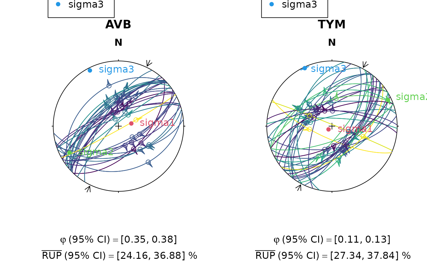
set.seed(20250411)

# Use Angelier examples:
nx <- length(angelier1990)
par(mfrow = c(2, nx/2))

invisible(lapply(seq_len(nx), function(i) {
  # inversion
  x <- angelier1990[[i]]
  res <- slip_inversion_michael(x, n_iter = 100, n = 1000, res = 100)

  # some stress shape
  phi_val <- round(res$phi_CI, 2)

  # misfit
  rup_val <- round(res$rup_CI, 2)

  # Plot the faults (color-coded by RUP%) and show the principal stress axes
  stereoplot(guides = FALSE)
  stereo_shmax(res$SHmax)
  fault_plot(x, col = assign_col(res$misfit$rup))
  stereo_confidence(res$principal_axes_CI$sigma1, col = 2)
  stereo_confidence(res$principal_axes_CI$sigma2, col = 3)
  stereo_confidence(res$principal_axes_CI$sigma3, col = 4)
  text(res$principal_axes, label = rownames(res$principal_axes), col = 2:4, adj = -.25)
  legend("topleft", col = 2:4, legend = rownames(res$principal_axes), pch = 16)
  title(
  main = names(angelier1990)[i],
  sub = bquote(atop(varphi ~ "(95% CI)" == "[" * .(phi_val[1]) * "," ~ .(phi_val[2]) * "]",
  ~ bar("RUP") ~ "(95% CI)" == "[" * .(rup_val[1]) * "," ~ .(rup_val[2]) * "] %")
  ))
}))