Fault Offsets

Tobias Stephan

2026-07-15

This tutorial demonstrates how you can derive displacement components from fault slip.

The offset along a fault can be factorized into several components.

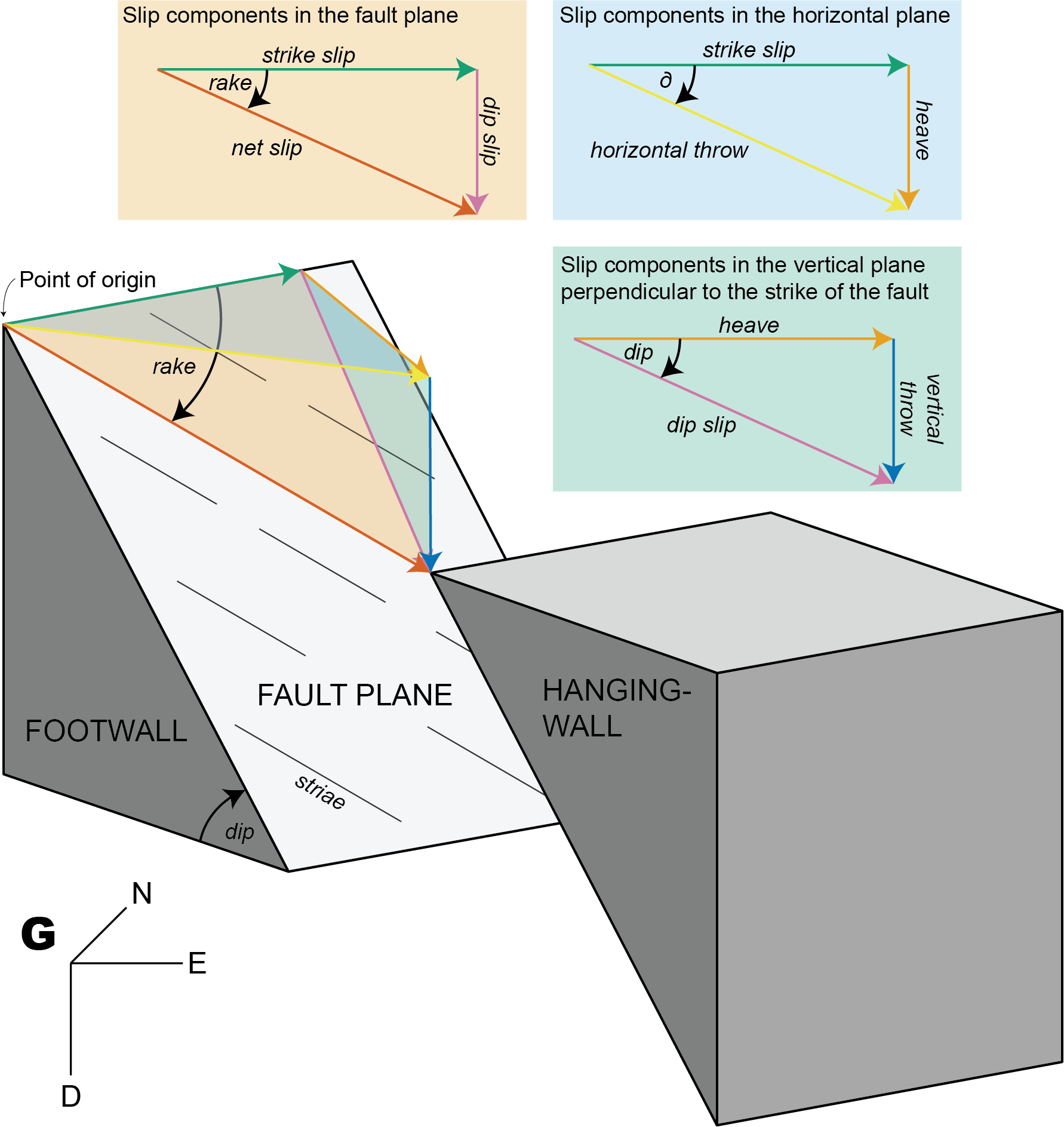
Fig. 1: Graphic illustration of displacement components along a fault. $\mathbb{G}$ as the georeference frame with D = down, E = East, N = North.

Get different components with trigonometry

Fault orientation (dip angle, dip direction), shortening direction, and horizontal throw

Knowing the horizontal throw (e.g. from plate motion parameters), the remaining components of the displacements along a given fault are as follows.

$$\begin{equation}\delta = |\sigma_{\textrm{Hmax}} - (\textrm{dip direction}+90^{\circ})|\end{equation}$$

Slip components in the horizontal plane:

$$\begin{equation}\begin{split} f_\textrm{strike slip} & = |\cos{\delta} * f_\textrm{horizontal throw}|\\ f_\textrm{heave} & = \sqrt{f_\textrm{horizontal throw}^2 - f_\textrm{strike slip}^2} \end{split}\end{equation}$$

Slip components in the vertical plane perpendicular to the strike of the fault:

$$\begin{equation}\begin{split} f_\textrm{dip slip} &= \frac{f_\textrm{heave}}{cos{(\textrm{dip})}}\\ f_\textrm{vertical throw} &= \sqrt{f_\textrm{dip slip}^2 - f_\textrm{heave}^2} \end{split}\end{equation}$$

Slip components in the fault plane plane:

$$\begin{equation}\begin{split} f_\textrm{net slip} &= \sqrt{f_\textrm{strike slip}^2 + f_\textrm{dip slip}^2}\\ \textrm{rake} &= \arctan{\left(\frac{f_\textrm{dip slip}}{f_\textrm{strike slip}}\right)} \end{split}\end{equation}$$

Thus, the rake angle describes the ratio between the dip slip and the strike slip component.

Knowing the vertical throw (e.g. from thermochronology or petrology), the fault dip (?assumption), and the direction and amount of horizontal offset, the strike of the fault is as follows:

$$\begin{equation}\begin{split} f_\textrm{heave} &= f_\textrm{vertical throw} * \tan{(\textrm{dip})}\\ \delta &= \arcsin{\left(\frac{f_\textrm{heave}}{f_\textrm{horizontal throw}}\right)}\\ \textrm{strike} &= |\sigma_{\textrm{Hmax}} - \delta| \end{split}\end{equation}$$

Knowing the vertical throw (e.g. from thermochronology or petrology), the fault strike (geomorphology), and the direction and amount of horizontal offset, the dip of the fault is as follows:

$$\begin{equation}\begin{split} \delta &= |\sigma_{\textrm{Hmax}} - \textrm{strike}|\\ f_\textrm{heave} &= f_\textrm{horizontal throw} * \sin{\delta} \\ \textrm{dip} &= \arctan{\left(\frac{f_\textrm{heave}}{f_\textrm{vertical throw}}\right)} \end{split}\end{equation}$$

Knowing the vertical throw (e.g. from thermochronology or petrology) and the fault’s dip and rake, the horizontal offset, the horizontal throw, and the net-slip are as follows:

Fault displacement tensors

Each fault component is a vector describing its direction and length. For instance, the vector of the strike slip is:

$$\begin{equation} \vec{f_\text{strike slip}} = \begin{pmatrix} \lVert f_\textrm{strike-slip}\rVert \\ 0 \\ 0 \end{pmatrix} \end{equation}$$

Net slip vector

Net slip vector

$$\begin{equation} \vec{f_\text{net}} = \begin{pmatrix} \lVert f_\textrm{strike-slip}\rVert \\ \lVert f_\textrm{heave}\rVert \\ \lVert f_\textrm{vertical throw}\rVert \end{pmatrix} \end{equation}$$

fault_displacements(strikeslip = 2, verticalthrow = -5, heave = 3)

Principal displacement tensor

The Eigen values of $\mathsf{F}_{ij}$; represented as $\{ \vec{f_1}, \vec{f_2}, \vec{f_3} \}$ are referred to as the heave, strike slip, and vertical throw component, respectively. These orthonormal vectors define a orthogonal matrix, i.e. the principal displacement tensor $\mathsf{F}_\mathbb{F}$:

$$\begin{equation}\mathsf{F}_{\mathbb{F}} = {\begin{bmatrix} \lVert f_\textrm{heave}\rVert & 0 & 0\\ 0 & \lVert f_\textrm{strike-slip}\rVert & 0\\ 0 & 0 & \lVert f_\textrm{vertical throw}\rVert\end{bmatrix}}\end{equation}$$

The tensor $\mathsf{F}$ can also be defined by the magnitudes of the fault displacements:

Fu <- displacement_tensor(s = 2, v = -5, h = 3)
print(Fu)

##      [,1] [,2] [,3]
## [1,]    3    0    0
## [2,]    0    2    0
## [3,]    0    0   -5
## attr(,"class")
## [1] "matrix"  "array"   "ftensor"

Orientation tensor

Fault orientation tensor is defined by the fault plane’s location, orientation (dip direction and dip angle), and the fault’s slip (direction and magnitude):

$$\begin{equation}\mathsf{F}_{ij} = {\begin{bmatrix}f_{11} & f_{12} & f_{13}\\ f_{21} & f_{22} & f_{23}\\ f_{31} & f_{32} & f_{33}\end{bmatrix}}\end{equation}$$

Fg <- displacement_tensor(s = 2, v = -5, h = 3, dip_direction = 45)
print(Fg)

##         [,1]      [,2] [,3]
## [1,] 2.12132  1.414214    0
## [2,] 2.12132 -1.414214    0
## [3,] 0.00000  0.000000   -5
## attr(,"class")
## [1] "matrix"  "array"   "ftensor"

From Principal displacement tensor to Orientation tensor

Translation point of origin in $\mathsf{F_\mathbb{F}}$ into point of measurement and rotate into fault orientation $\mathsf{F}_\mathbb{FG}$

displacement_tensor_decomposition(Fg, dip_direction = 45)

## $displacements
##           dip    delta     rake verticalthrow horizontalthrow heave  dipslip
## [1,] 59.03624 56.30993 71.06818            -5        3.605551     3 5.830952
##      strikeslip  netslip
## [1,]          2 6.164414
## 
## $fault
## Fault object (n = 1):
## dip_direction           dip       azimuth        plunge         sense 
##      45.00000      59.03624     258.69007     -54.20424      -1.00000 
## 
## $strain_tensor
##      [,1] [,2] [,3]
## [1,]  3.0 -1.5 -1.5
## [2,] -1.0  1.0 -1.0
## [3,]  2.5  2.5 15.0
## 
## $volumetric_strain
## [1] 19
## 
## $shear_strain
## [1] 5.196152