9D Direct Inversion for Fault Slip Including Vorticity

Direct inversion of stress, strain or strain rate including vorticity using 9D parameter space using the method by Hansen (2013). It can be applied regardless whether the dynamic or the kinematic hypothesis is adopted; it can handle datasets representing two to seven degrees of freedom; and it is not dependent on the correct assessment of slip sense.

Usage

slip_inversion_hansen(x, flip = FALSE, friction = 0.6, type = c("9d", "6d"))

Arguments

x: object of class "Pair" or "Fault" with at least 7 rows.
flip: logical. Flip if you want to have the negative stress tensor, i.e. sigma 1 and 3 will be flipped.
friction: numeric. Coefficient of friction (0.6 by default)
type: character. Inversion method, either "9d" (the default) for using the 9-dimensional or "6d" for the 6-dimensional parameter space.

Value

list. See slip_inversion_michael() for output description. If type == '9d, additional outputs are the vorticity axis ("vorticity_axis", a Vec3 object) and the magnitude of vorticity ("vorticity_mag", a numeric).

list

Details

If no vorticity is involved, the inversion can be done by using a 6-dimensional parameter space only (type = '6d').

References

Hansen, J. A. (2013). Direct inversion of stress, strain or strain rate including vorticity: A linear method of homogenous fault-slip data inversion independent of adopted hypothesis. Journal of Structural Geology, 51, 3–13. https://doi.org/10.1016/j.jsg.2013.03.014

Examples

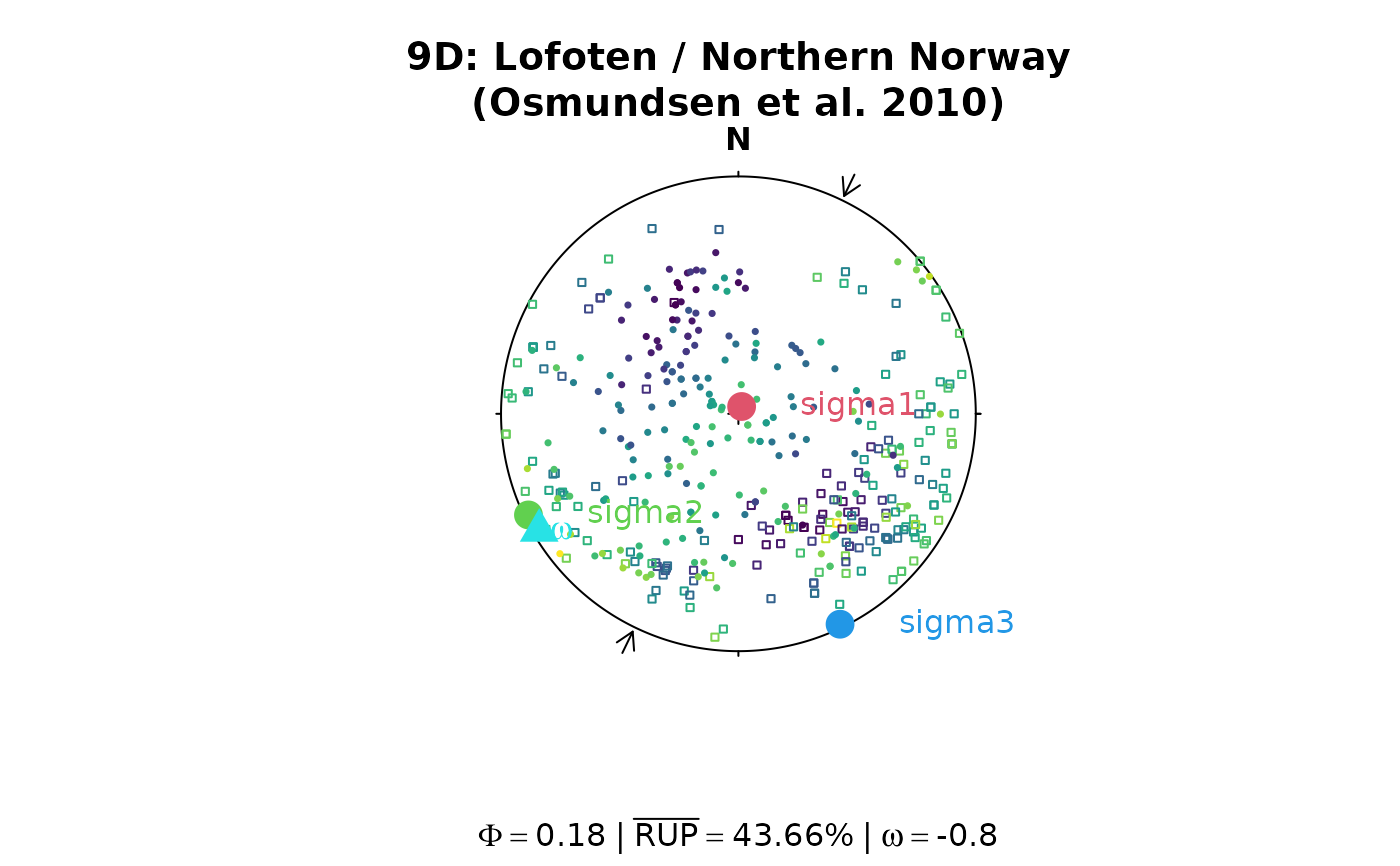
# Osmundsen et al. 2010 dataset
## 9D solution
res <- slip_inversion_hansen(osmundsen2010, flip = TRUE)

phi_val <- round(res$stress_shape$phi, 2)
rup_val <- round(res$misfit$rup, 2)
w_val <- round(res$vorticity_mag, 2)

stereoplot(title = "9D: Lofoten / Northern Norway\n(Osmundsen et al. 2010)", guides = FALSE)
stereo_shmax(res$SHmax)
points(Plane(osmundsen2010), col = assign_col(res$misfit$rup), pch = 0, cex = 0.5)
points(Line(osmundsen2010), col = assign_col(res$misfit$rup), pch = 16, cex = 0.5)
points(res$principal_axes, col = 2:4, pch = 16, cex = 2)
text(res$principal_axes, labels = rownames(res$principal_axes), col = 2:4, adj = -.5)
points(res$vorticity_axis, col = 5, pch = 17, cex = 2)
text(res$vorticity_axis, labels = bquote(omega), col = 5, adj = -.5)

title(sub = bquote(Phi == .(phi_val) ~ "|" ~ bar("RUP") == .(rup_val) * "%" ~
  "|" ~ omega == .(w_val)))


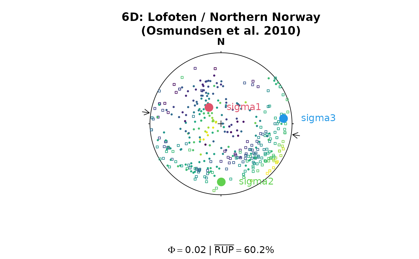
## 6D inversion
res6 <- slip_inversion_hansen(osmundsen2010, flip = TRUE, type = "6d")

phi6_val <- round(res6$stress_shape$phi, 2)
rup6_val <- round(res6$misfit$rup, 2)

stereoplot(title = "6D: Lofoten / Northern Norway\n(Osmundsen et al. 2010)", guides = FALSE)
stereo_shmax(res6$SHmax)
points(Plane(osmundsen2010), col = assign_col(res6$misfit$rup), pch = 0, cex = 0.5)
points(Line(osmundsen2010), col = assign_col(res6$misfit$rup), pch = 16, cex = 0.5)
points(res6$principal_axes, col = 2:4, pch = 16, cex = 2)
text(res6$principal_axes, labels = rownames(res6$principal_axes), col = 2:4, adj = -.5)

title(sub = bquote(Phi == .(phi6_val) ~ "|" ~ bar("RUP") == .(rup6_val) * "%"))


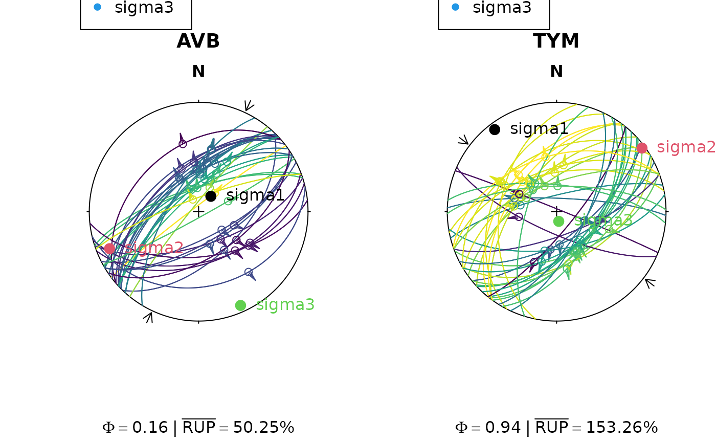
# Angelier 1990 dataset
nx <- length(angelier1990)
par(mfrow = c(1, nx))

invisible(lapply(seq_len(nx), function(i) {
  # inversion
  x <- angelier1990[[i]]
  res <- slip_inversion_hansen(x, type = "6d")

  # some stress shape
  phi_val <- round(res$stress_shape$phi, 2)

  # misfit
  rup_val <- round(res$misfit$rup_mean, 2)

  # Plot the faults (color-coded by RUP%) and show the principal stress axes
  stereoplot(title = names(angelier1990)[i], guides = FALSE)
  stereo_shmax(res$SHmax)
  fault_plot(x, col = assign_col(res$misfit$rup))
  points(res$principal_axes, col = 1:3, pch = 16, cex = 1.5)
  text(res$principal_axes,
    label = rownames(res$principal_axes),
    col = 1:3, adj = -.25
  )
  legend("topleft", col = 2:4, legend = rownames(res$principal_axes), pch = 16)
  title(sub = bquote(Phi == .(phi_val) ~ "|" ~ bar("RUP") == .(rup_val) * "%"))
}))