
Stress tensor inversion via the Yamaji and Sato (2006) eigenvector method.
Source:R/stress_inversion_yamaji.R
slip_inversion_yamaji_sato.RdStress tensor inversion via the Yamaji and Sato (2006) eigenvector method.
Value
Same output as slip_inversion() plus
y6D unit y-vector on S^5 representing the tensor
alphaper-fault angular misfit (unsigned, 0-90°)
mean_alphamean angular misfit across all faults
References
Yamaji, A., & Sato, K. (2006). Distances for the solutions of stress tensor inversion in relation to misfit angles that accompany the solutions. Geophysical Journal International, 167(2), 933–942. doi:10.1111/j.1365-246X.2006.03188.x
See also
Other stress-inversion:
Fault_PT(),
slip_inversion(),
slip_inversion_angelier(),
slip_inversion_hansen(),
slip_inversion_michael(),
slip_inversion_simple(),
slip_inversion_wissi()
Other yamaji:
slip_inversion_yamaji_sato_boot()
Examples
set.seed(20250411)
nx <- length(angelier1990)
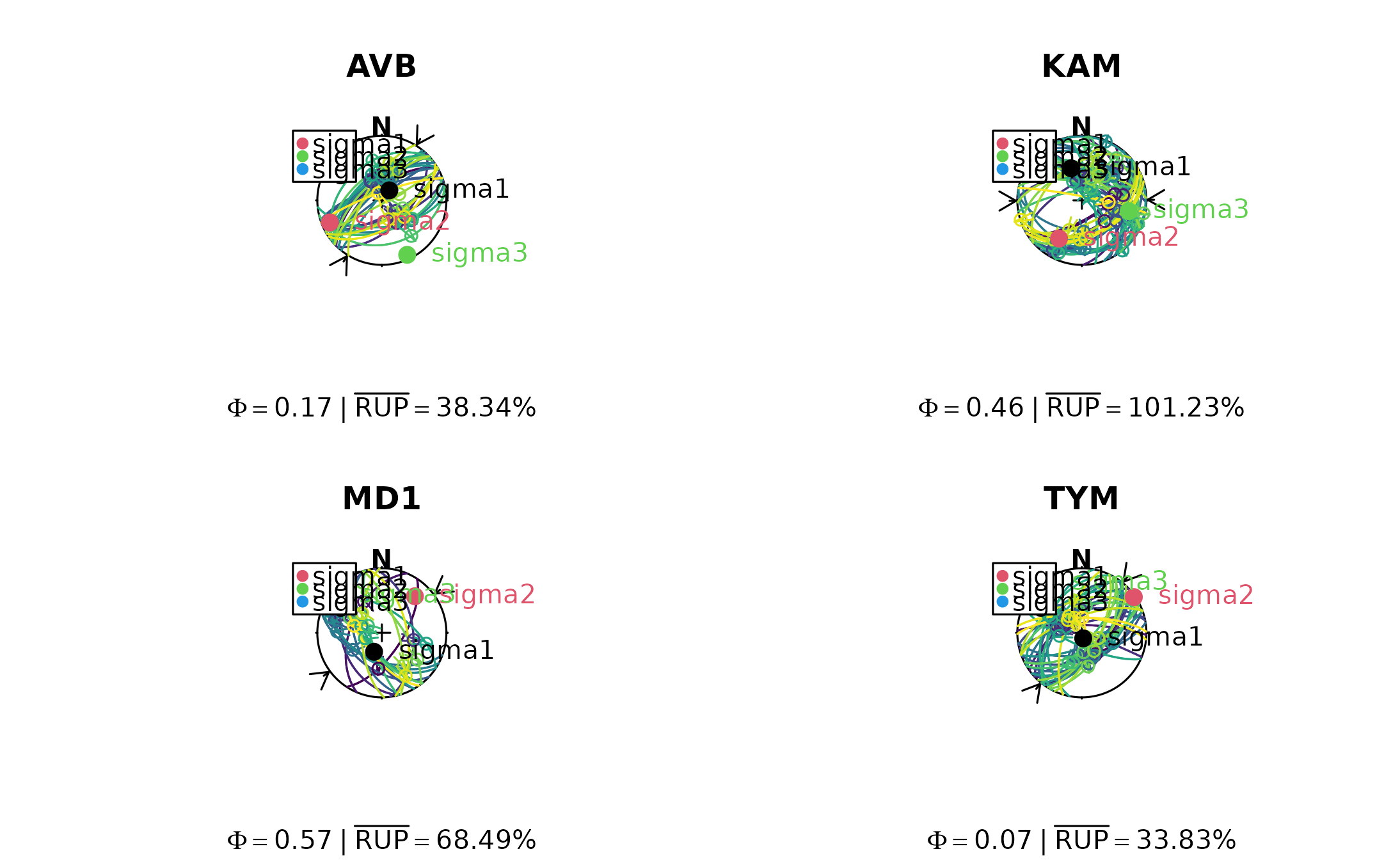
par(mfrow = c(2, nx/2))
invisible(lapply(seq_len(nx), function(i) {
# inversion
x <- angelier1990[[i]]
res <- slip_inversion_yamaji_sato(x)
# some stress shape
phi_val <- round(res$stress_shape$phi, 2)
# misfit
rup_val <- round(res$misfit$rup_mean, 2)
# Plot the faults (color-coded by RUP%) and show the principal stress axes
stereoplot(title = names(angelier1990)[i], guides = FALSE)
stereo_shmax(res$SHmax)
fault_plot(x, col = assign_col(res$misfit$rup))
points(res$principal_axes, col = 1:3, pch = 16, cex = 1.5)
text(res$principal_axes,
label = rownames(res$principal_axes),
col = 1:3, adj = -.25
)
legend("topleft", col = 2:4, legend = rownames(res$principal_axes), pch = 16)
title(sub = bquote(Phi == .(phi_val) ~ "|" ~ bar("RUP") == .(rup_val) * "%"))
}))
 dev.off()
#> null device
#> 1
dev.off()
#> null device
#> 1