Orientation Plots • structr

This tutorial shows how to create various orientation plots using the {structr} package, including stereographic and equal-area projections, fabric plots, density plots, and fault plots.

library(structr)

Import and convert to spherical objects:

data(example_planes_df)
data(example_lines_df)

planes <- Plane(example_planes_df$dipdir, example_planes_df$dip)
lines <- Line(example_lines_df$trend, example_lines_df$plunge)

Equal-area projection

Lambert equal area, lower hemisphere projection is the default plotting setting.

stereoplot(guides = TRUE)
points(lines, col = "#B63679", pch = 19, cex = .5)
points(planes, col = "#000004", pch = 1, cex = .5)

legend("topright", legend = c("Lines", "Planes"), col = c("#B63679", "#000004"), pch = c(19, 1), cex = 1)
title(main = "Example data", sub = "Lambert equal area, lower hemisphere projection")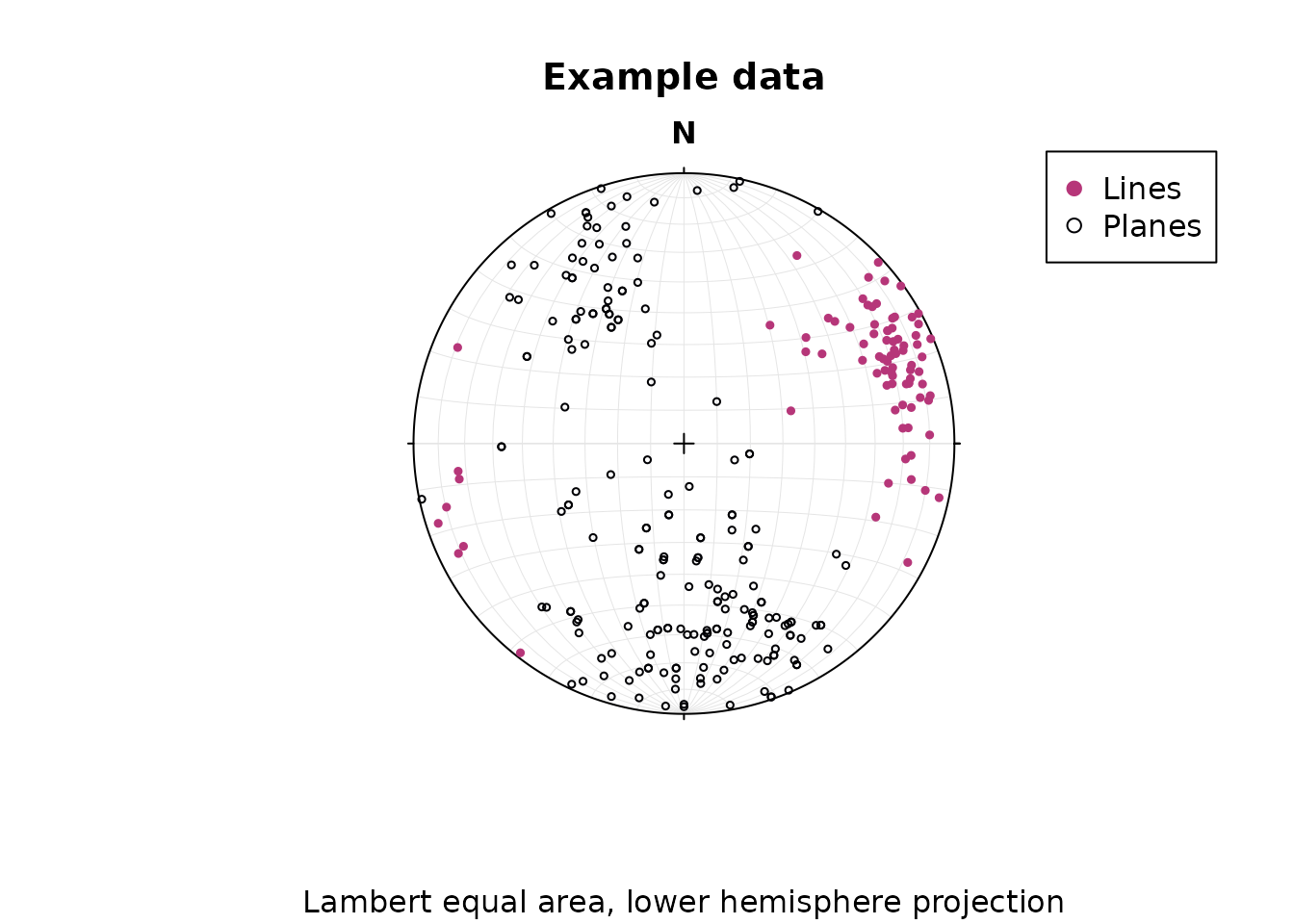

Diagram showing the equal-area Lambert projection of some example data

Tip

Points can be added using the points() function.

Stereographic projection

To change to equal angle stereographic, upper hemisphere projection, just set the earea argument to FALSE, and the upper.hem argument to TRUE:

stereoplot(earea = FALSE, guides = TRUE)
points(lines, col = "#B63679", pch = 19, cex = .5, earea = FALSE, upper.hem = TRUE)
points(planes, col = "#000004", pch = 1, cex = .5, earea = FALSE, upper.hem = TRUE)

legend("topright", legend = c("Lines", "Planes"), col = c("#B63679", "#000004"), pch = c(19, 1), cex = 1)
title(main = "Example data", sub = "Equal angle stereographic, upper hemisphere projection")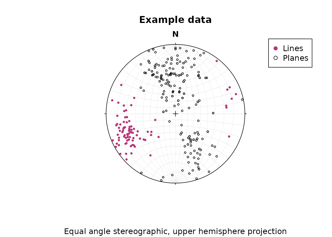

Diagram showing the equal-angle stereographic projection of some example data

Tip

Global plotting settings can be defined using options(). This is useful when you want to create several plots using the same plotting parameters. For example, to turn off guides:

options(structr.guides = FALSE)

Great and small circles

Great and small circles can be added using the lines() function.

Adding great circles for the first 10 vectors in planes:

stereoplot()
lines(planes[1:10, ], col = "lightgrey", lty = 1)
points(planes[1:10, ], col = "#000004", pch = 1, cex = .5)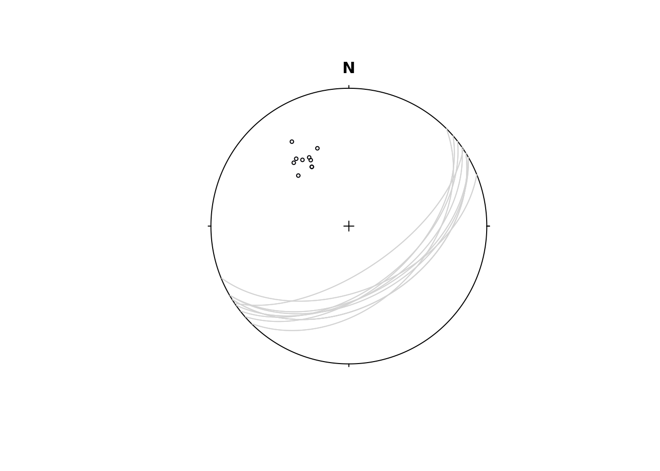

To plot a small circle with, e.g., a 10° radius, you need to specify the ang argument in lines():

stereoplot()
lines(lines[1:5, ], ang = 10, col = "#B6367980", border = "#B63679", fill = TRUE)
points(lines[1:5, ], col = "#B63679", pch = 19, cex = .5)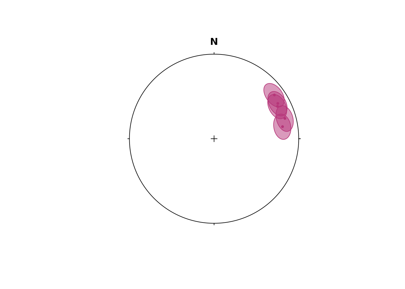

Pair Objects (Linear Element on a Plane)

Pair objects contain plane and line measurements, such as stretching lineations on foliation planes, or intersection lineations on bedding planes etc.

data(strabo_prj)
my_pairs <- structr::Pair(strabo_prj$planar, strabo_prj$linear)

plot(my_pairs, col = assign_col_d(strabo_prj$data$spot_id))
#> Warning in (function (n) : This manual palette can handle a maximum of 8
#> values. You have supplied 93
title("Pairs")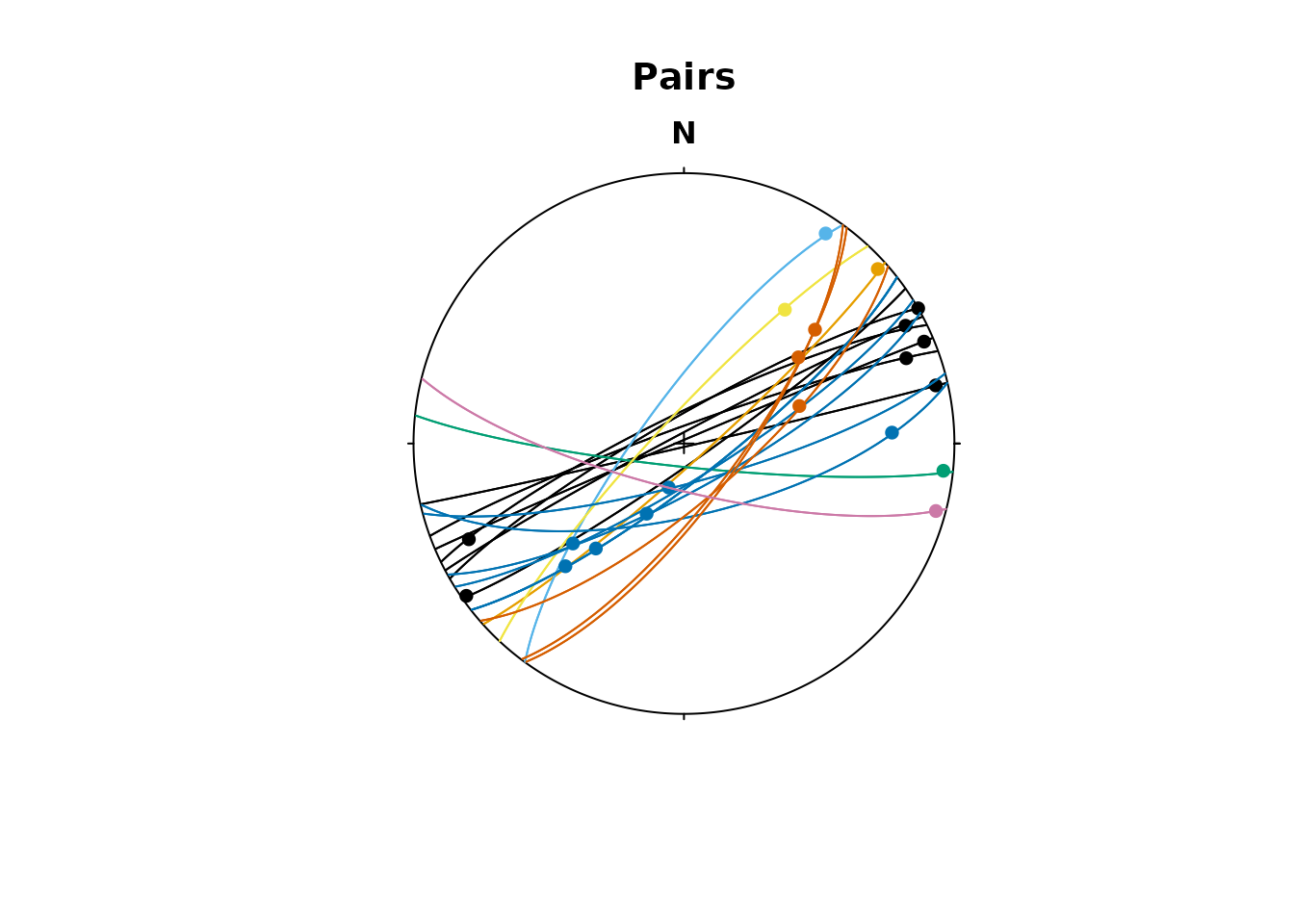

Diagram showing plane-line pairs from a StraboSpot project, colored by spot

Dip-Pitch-Plunge Ternary diagram

The Dip-Pitch-Plunge Diagram is a ternary fabric orientation diagram after Balé and Brun (1989)¹ using the pitch and plunge of stretching lineation (X) and the dip of the foliation plane (XY). This can be used to show three-dimensional geometries of fabrics (useful for transpression).

balebrun_plot(my_pairs, col = assign_col_d(strabo_prj$data$spot_id), pch = 16)
#> Warning in (function (n) : This manual palette can handle a maximum of 8
#> values. You have supplied 93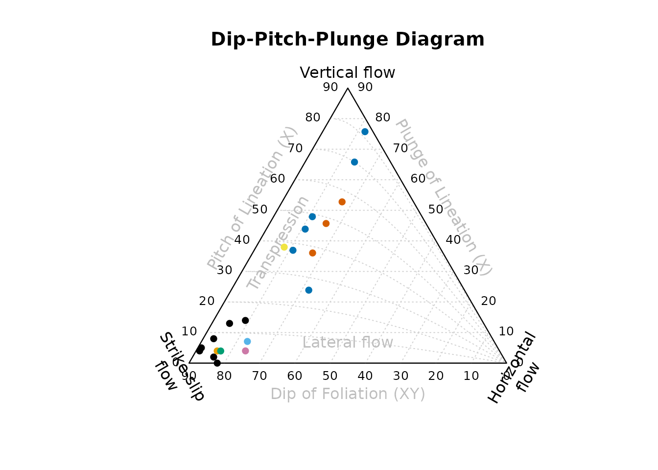

Ternary dip-pitch-plunge diagram of the plane-line pairs after Balé and Brun 1989

Fabric plots

The Eigenvalues of the orientation tensor describe the shape of the distribution of these vectors, that is how clustered, cylindrical or random these vectors are distributed.

A Fabric plot visualizes the shape of the distribution by plotting the eigenvalues of the orientation tensor. Three different diagrams are provided by {structr}, namely the triangular Vollmer plot², the logarithmic biplot (Woodcock plot)³, and the Lode parameter vs. natural octahedral strain diagram (Hsu plot)⁴.

Vollmer plot

vollmer_plot() creates a triangular plot showing the shape of the orientation distribution (after Vollmer, 1990).

vollmer_plot(planes, col = "#000004", pch = 1, cex = 2, guides = TRUE)
vollmer_plot(lines, add = TRUE, col = "#B63679", pch = 19, cex = 2)
legend("topright", legend = c("Lines", "Planes"), col = c("#B63679", "#000004"), pch = c(19, 1), cex = 1)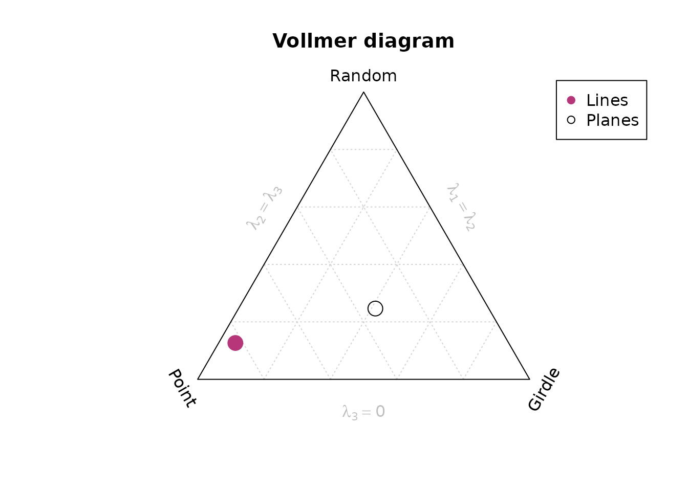

Diagram showing eigen-vector analysis of some example data plotted in a triangular plot after Vollmer 1990

Woodcock plot

woodcock_plot() creates a logarithmic biplot showing the shape of the orientation distribution (after Woodcock, 1977).

woodcock_plot(planes, col = "#000004", pch = 1, cex = 2, guides = TRUE)
woodcock_plot(lines, add = TRUE, col = "#B63679", pch = 19, cex = 2)
legend("topright", legend = c("Lines", "Planes"), col = c("#B63679", "#000004"), pch = c(19, 1), cex = 1)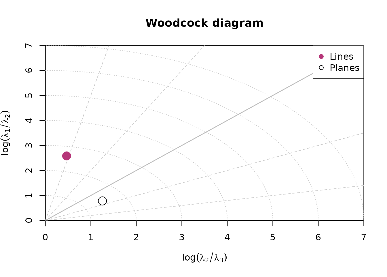

Diagram showing eigen-vector analysis of some example data plotted in a logarithmic biplot after Woodcock 1977

Hsu plot

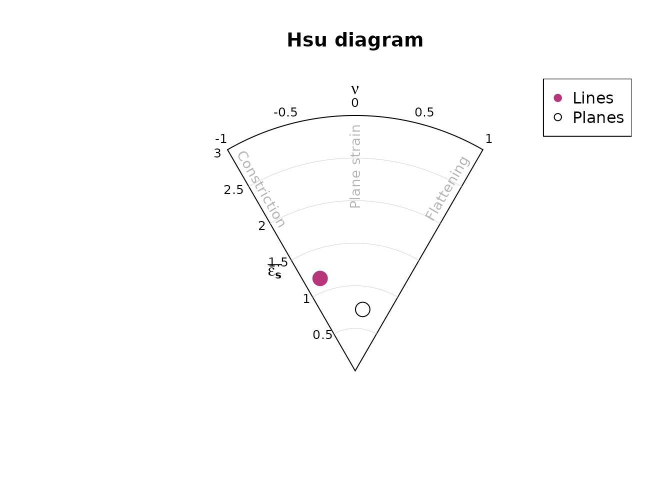
hsu_plot() creates a Lode parameter⁵ vs. natural octahedral strain⁶ diagram showing the shape of the orientation distribution (after Hsu, 1966).

hsu_plot(planes, col = "#000004", pch = 1, cex = 2, guides = TRUE)
hsu_plot(lines, add = TRUE, col = "#B63679", pch = 19, cex = 2)
legend("topright", legend = c("Lines", "Planes"), col = c("#B63679", "#000004"), pch = c(19, 1), cex = 1)

Diagram showing eigen-vector analysis of some example data plotted in a Hsu plot

Density plots

Kamb contours⁷ and densities can be added to an existing projection plot using the contour functions. Weighted densities can be controlled by the weights argument and are useful when the orientation measurements have different accuracies.

example_planes_df$quality <- ifelse(is.na(example_planes_df$quality), 6, example_planes_df$quality) # replacing NA values with 6
plane_weightings <- 6 / example_planes_df$quality

stereoplot()
points(planes, col = "grey", pch = 16, cex = .5)
contour(planes, add = TRUE, density.params = list(weights = plane_weightings))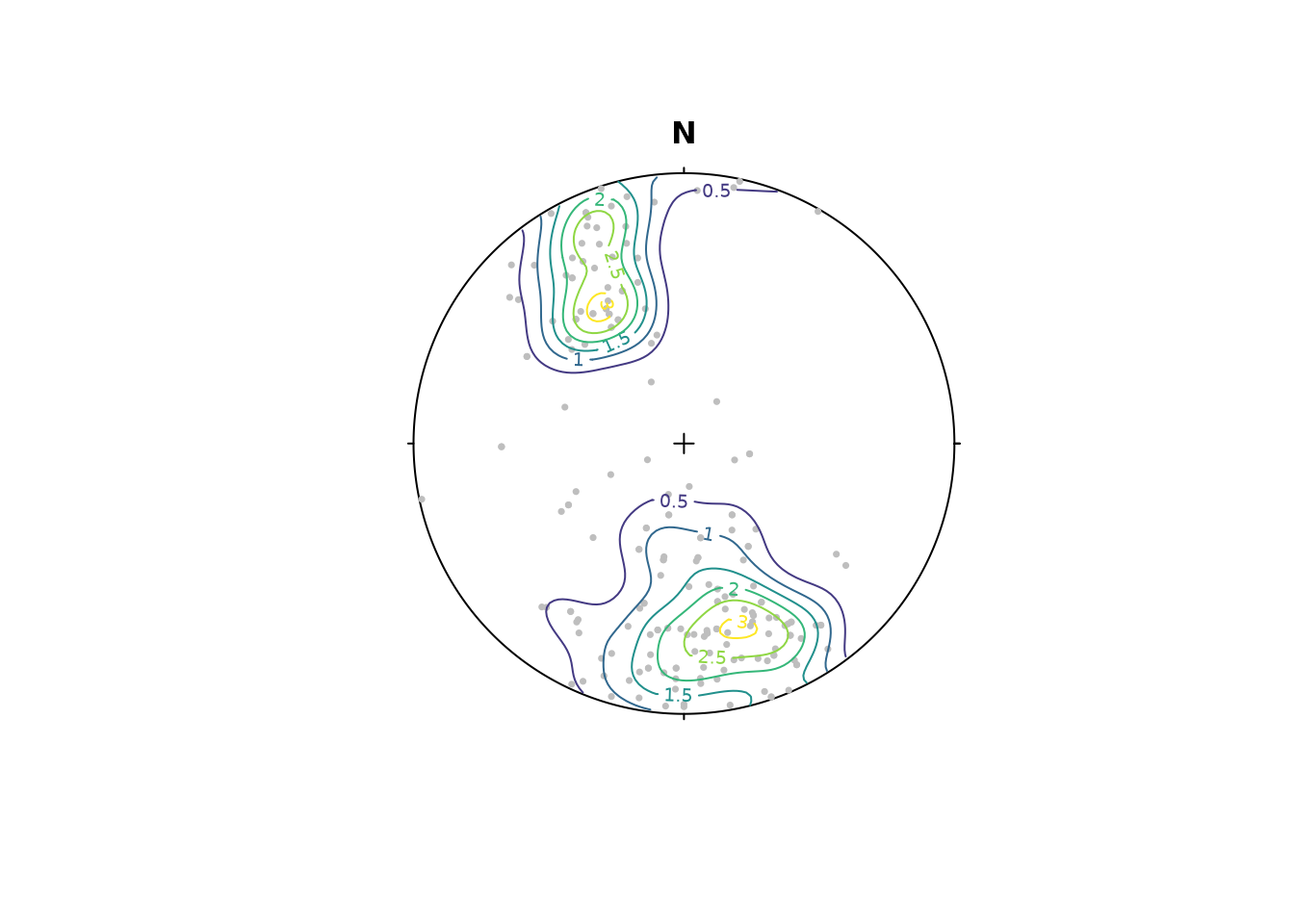

Diagram showing the density distribution of some example data plotted in an equal-area projection

contour() adds contour lines, while contourf() adds filled contours and image() adds a density image (i.e. a dense grid of colored rectangles). See ?contour, ?contourf, and ?image for more information.

stereoplot()
points(planes, col = "grey", pch = 16, cex = .5)
contourf(planes, add = TRUE, density.params = list(weights = plane_weightings))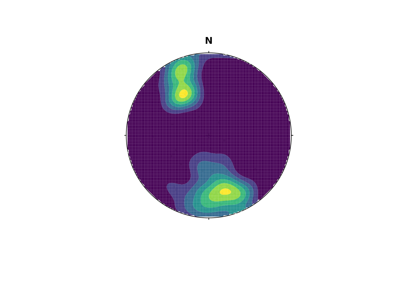

Diagram showing the filled density distribution of some example data plotted in an equal-area projection

Synopsis

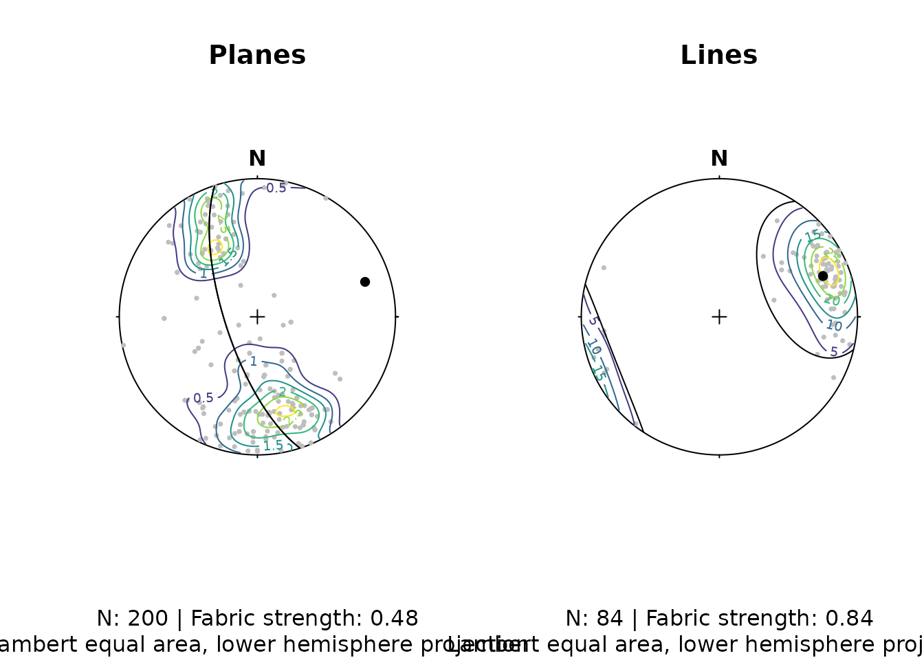
Let’s create a publication ready synoptical plot for the line and plane orientation data, showing the density distribution, eigenvectors/mean values, and fabric strength.

# Minimum eigenvector of plane's orientation tensor:
planes_eigen <- ot_eigen(planes)$vectors
planes_eigen3 <- planes_eigen[3, ]

# Mean and SD of lines
lines_mean <- sph_mean(lines)
lines_sd <- sph_sd(lines)

# Fabric strength
fabric_p <- vollmer(planes)["D"]
fabric_l <- vollmer(lines)["D"]

The final plot:

# two plots side by side
par(mfrow = c(1, 2))

# Planes
stereoplot()
points(planes, col = "grey", pch = 16, cex = .5)
contour(planes, add = TRUE, density.params = list(weights = plane_weightings))
points(planes_eigen3, col = "black", pch = 16)
lines(planes_eigen3, col = "black", pch = 16)
title(
  main = "Planes",
  sub = paste0(
    "N: ", nrow(planes), " | Fabric strength: ", round(fabric_p, 2),
    "\nLambert equal area, lower hemisphere projection"
  )
)

# Lines
stereoplot()
points(lines, col = "grey", pch = 16, cex = .5)
contour(lines, add = TRUE)
points(lines_mean, col = "black", pch = 16)
lines(lines_mean, ang = lines_sd, col = "black")
title(
  main = "Lines",
  sub = paste0(
    "N: ", nrow(lines), " | Fabric strength: ", round(fabric_l, 2),
    "\nLambert equal area, lower hemisphere projection"
  )
)

Diagram showing the density distribution, eigenvectors and mean values

Fault plots

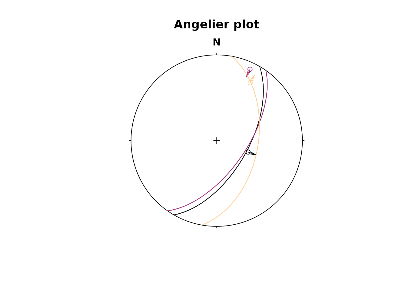
Fault objects consist of planes (fault plane), lines (e.g. striae), and the sense of movement. There are two ways how these combined features can be visualized, namely the Angelier and the Hoeppener plot.

Angelier plot

The Angelier plot shows all planes as great circles and lineations as points (after Angelier, 1984)⁸. Fault striae are plotted as vectors on top of the lineation pointing in the movement direction of the hanging wall. Easy to read in case of homogeneous or small datasets.

f <- Fault(
  c("a" = 120, "b" = 125, "c" = 100),
  c(60, 62, 50),
  c(110, 25, 30),
  c(58, 9, 23),
  c(1, -1, 1)
)

stereoplot(title = "Angelier plot")
angelier(f, col = viridis::magma(nrow(f), end = .9))

Diagram showing example fault data plotted in an equal-area projection

Hoeppener plot

The Hoeppener plot shows all planes as poles while lineations are not shown (after Hoeppener, 1955)⁹. Instead, fault striae are plotted as vectors on top of poles pointing in the movement direction of the hanging wall. Useful in case of large or heterogeneous datasets.

stereoplot(title = "Hoeppener plot")
hoeppener(f, col = viridis::magma(nrow(f), end = .9), points = FALSE)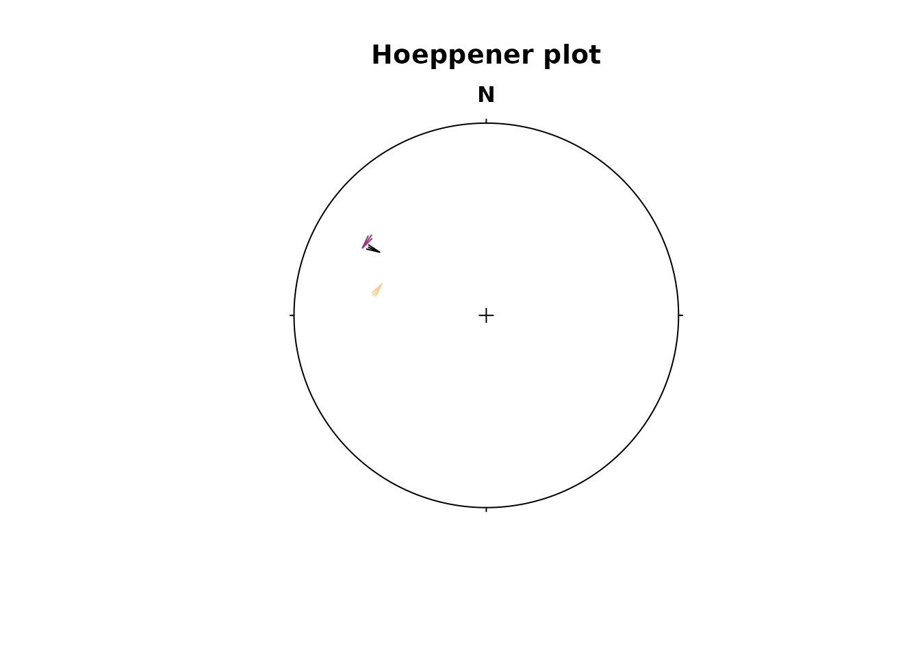

The points argument disables plotting the points at the start of the arrows.

Note

fault_plot() is a wrapper function that allows to switch between Angelier and Hoeppener plot using the type argument. See ?fault_plot for details.

Assign plotting parameters based on data

{structr} offers some convenience functions to help you map certain plotting parameters such as color, size, and symbol based on vector values:

assign_col() for color
assign_cex() for marker size (character expansion)
assign_pch() for marker symbols (plotting character)

The following example assigns the col (color), the cex (size), and the pch (symbol) based on three different properties:

# define three random properties
prop_continuous1 <- runif(nrow(planes))
prop_continuous2 <- runif(nrow(planes))
prop_discrete <- sort(letters[sample(1:3, size = nrow(planes), replace = TRUE)])

stereoplot()
points(planes,
  col = assign_col(prop_continuous1),
  cex = assign_cex(prop_continuous2, area = TRUE),
  pch = assign_pch(prop_discrete)
)

# Add legends
legend_cex(prop_continuous2, area = TRUE, title = "A continuous property", position = "bottomleft", cex = .8)
legend_pch(prop_discrete, title = "A discrete property", position = "topleft", cex = .8)
legend_col(pretty(prop_continuous1), title = "Another continuous property")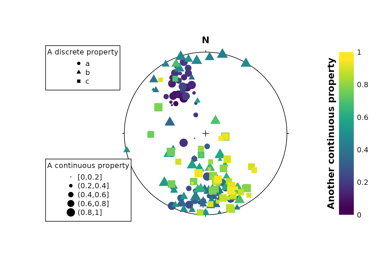

Diagram showing planes with color, size and symbol mapped to three properties

The legend for these plotting parameters can be created using the legend_* functions.

The assign_* functions work on continuous values; for discrete values use the assign_*_d variants, and for binned mapping use assign_*_binned. See ?assign_cex() for more information.