
This tutorial demonstrates geodesic regression, a method to determine statistically the best-fit great- or small-circle for a set of vectors.
Import some example data of some folded fabric elements:
data("gray_example")
gray_example
#> Plane object (n = 16):
#>          dip_direction dip
#> Cleavage           232  58
#> Cleavage           245  63
#> Cleavage           256  82
#> Cleavage            87  83
#> Cleavage            99  68
#> Cleavage           101  60
#> Cleavage           107  48
#> Cleavage           240  65
#> Bedding            246  50
#> Bedding            236  45
#> Bedding            228  34
#> Bedding            188  33
#> Bedding            152  36
#> Bedding            133  48
#> Bedding            124  48
#> Bedding            119  61
Show data in equal-area projection:
cleavage <- gray_example[1:8, ]
bedding <- gray_example[9:16, ]

stereoplot()
points(cleavage, col = "#1D1147")
points(bedding, col = "#E65164", pch = 4)

legend("topright", col = c("#1D1147", "#E65164"), pch = c(1, 4), legend = c("Poles to cleavage", "Poles to bedding"), bg = "white")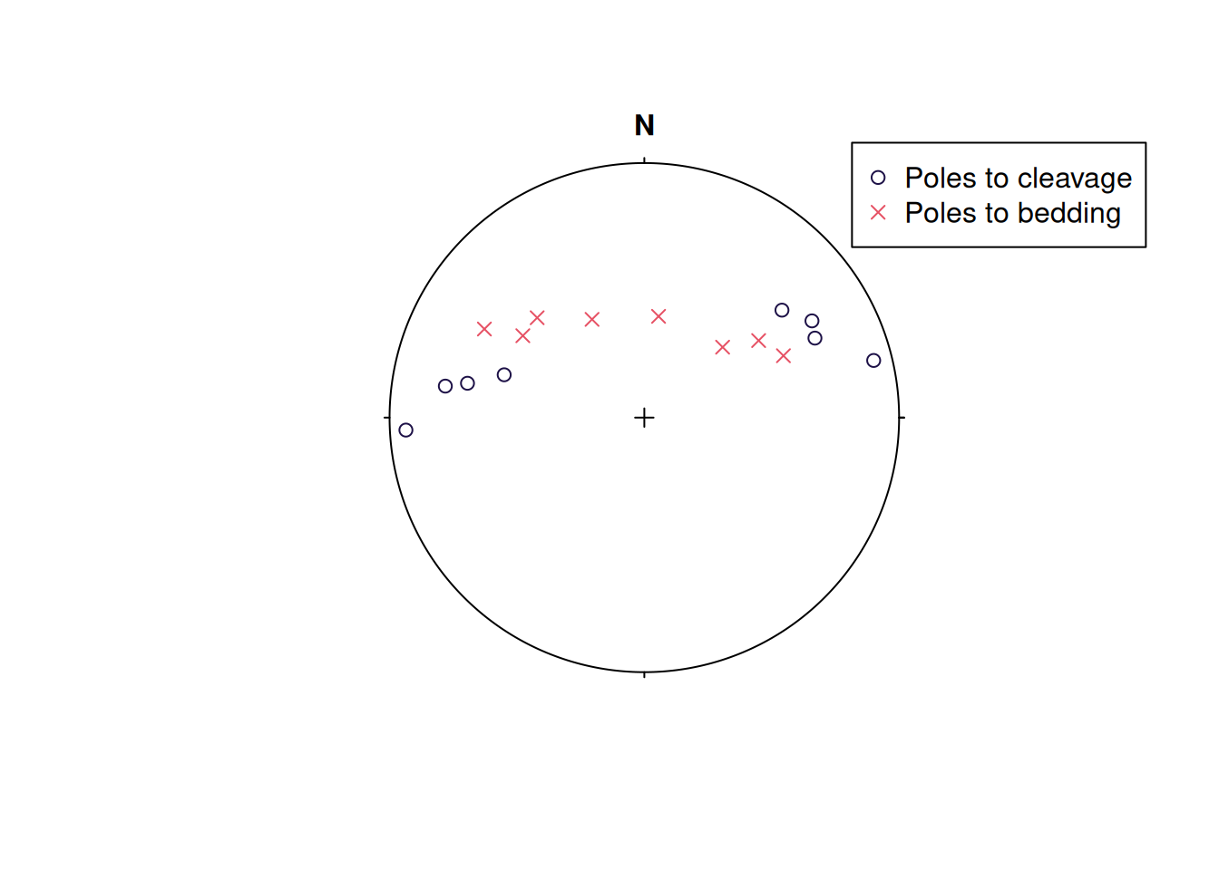
The diagram suggests that both the cleavage and the bedding poles are distributed along great circles or small circles. To find the orientation of the axes of these circles, and to decide whether the poles better fit a great- or a small-circle solution, we’ll perform a (geodesic) regression. For poles to folded bedding, the axis of a best-fit great circle is the fold axis of a cylindrical fold (π-diagram), whereas a small-circle arrangement is expected for conical folds or fanning cleavage.
Best-fit great circles
First, we determine the best-fit great circle for the two fabric elements. The great-circle regression is done via regression_greatcircle(), which returns a list containing the axis of the great circle:
cleavage_gc <- regression_greatcircle(cleavage)
bedding_gc <- regression_greatcircle(bedding)

# The axis of the great circles:
cleavage_gc$vec
#> Plane object (n = 1):
#> dip_direction           dip
#>     351.21775      57.37635
bedding_gc$vec
#> Plane object (n = 1):
#> dip_direction           dip
#>      6.893869     58.942197
The algorithm minimizes the sum of squares of the residuals, which are the angular distances of the data vectors from the best-fit circle (i.e. the deviation of each vector’s angle to the axis from 90° for a great circle, or from the cone angle for a small circle). We can check whether the optimization successfully converged to a minimum, and assess the quality of the fit using the R2:
# Check
cleavage_gc$convergence == 0 & cleavage_gc$min_eigenvalue > 0
#> [1] TRUE
bedding_gc$convergence == 0 & bedding_gc$min_eigenvalue > 0
#> [1] TRUE

# R^2 value
cleavage_gc$r_squared
#> [1] 0.5364717
bedding_gc$r_squared
#> [1] 0.9770348
Plot the results:
stereoplot()
lines(cleavage_gc$vec, col = "#000004FF")
lines(bedding_gc$vec, col = "#B63679")
points(cleavage, col = "#1D1147")
points(bedding, col = "#E65164", pch = 4)

legend("bottomright", col = c("#000004FF", "#B63679"), lty = c(1, 1), legend = c("Cleavage best great circle", "Bedding best great circle"), bg = "white")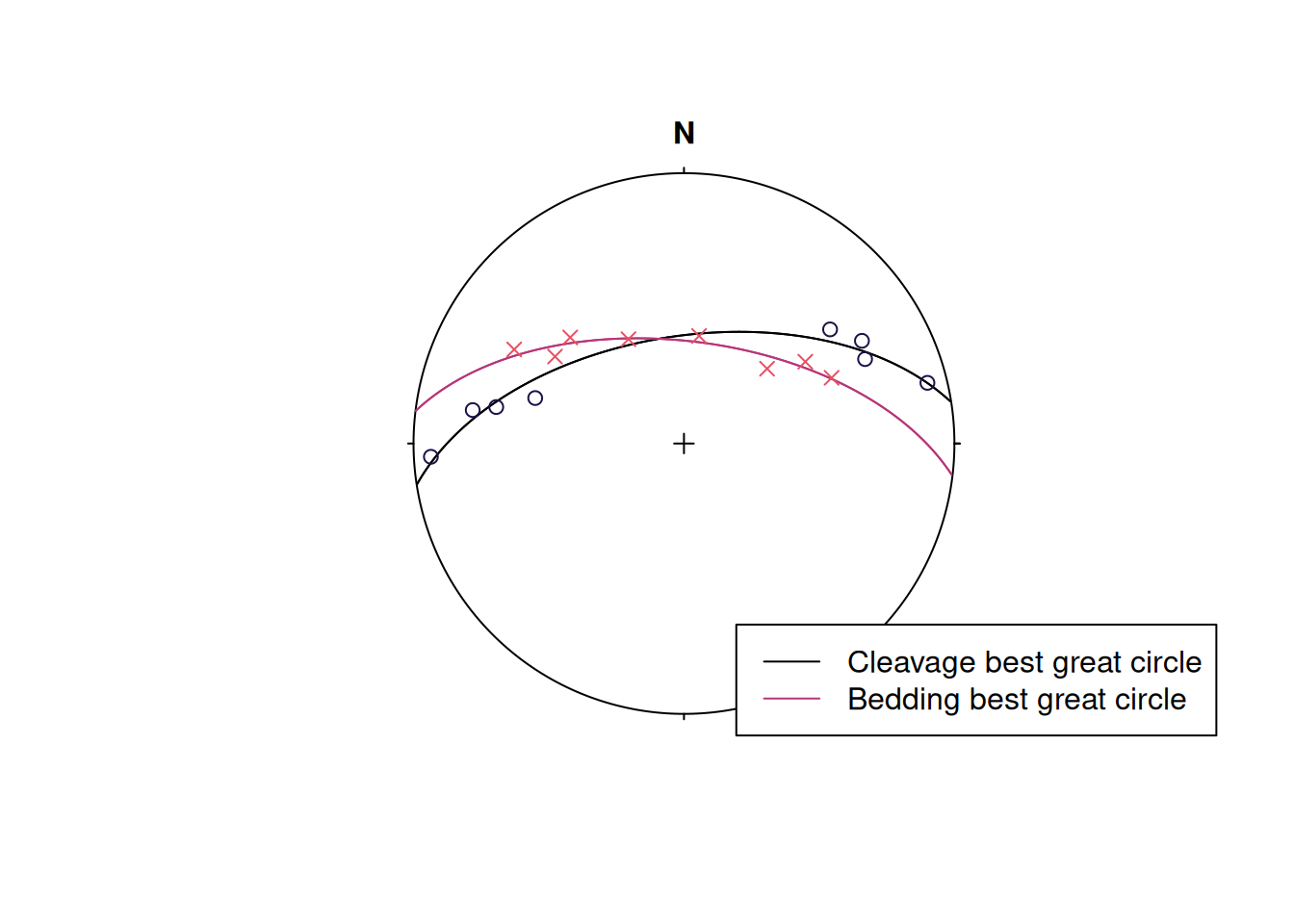
Summary
The regression was successful. However, the R2 values indicate a good fit for the bedding, but a rather poor fit for the cleavage.
Best-fit small circles
cleavage_sc <- regression_smallcircle(cleavage)
bedding_sc <- regression_smallcircle(bedding)

# Half-apical angle of small-circle cone (in degrees)
cleavage_sc$cone
#> [1] 88.58424
bedding_sc$cone
#> [1] 92.12321
Check the optimization convergence and the fit:
# Check
cleavage_sc$convergence == 0 & cleavage_sc$min_eigenvalue > 0
#> [1] TRUE
bedding_sc$convergence == 0 & bedding_sc$min_eigenvalue > 0
#> [1] TRUE

# R^2 value
cleavage_sc$r_squared
#> [1] 0.5368224
bedding_sc$r_squared
#> [1] 0.9771265
Plot the results:
stereoplot()
lines(cleavage_sc$vec, cleavage_sc$cone, col = "#000004FF")
lines(bedding_sc$vec, bedding_sc$cone, col = "#B63679")
points(cleavage, col = "#1D1147")
points(bedding, col = "#E65164", pch = 4)

legend("bottomright", col = c("#000004FF", "#B63679"), lty = c(1, 1), legend = c("Cleavage best small circle", "Bedding best small circle"), bg = "white")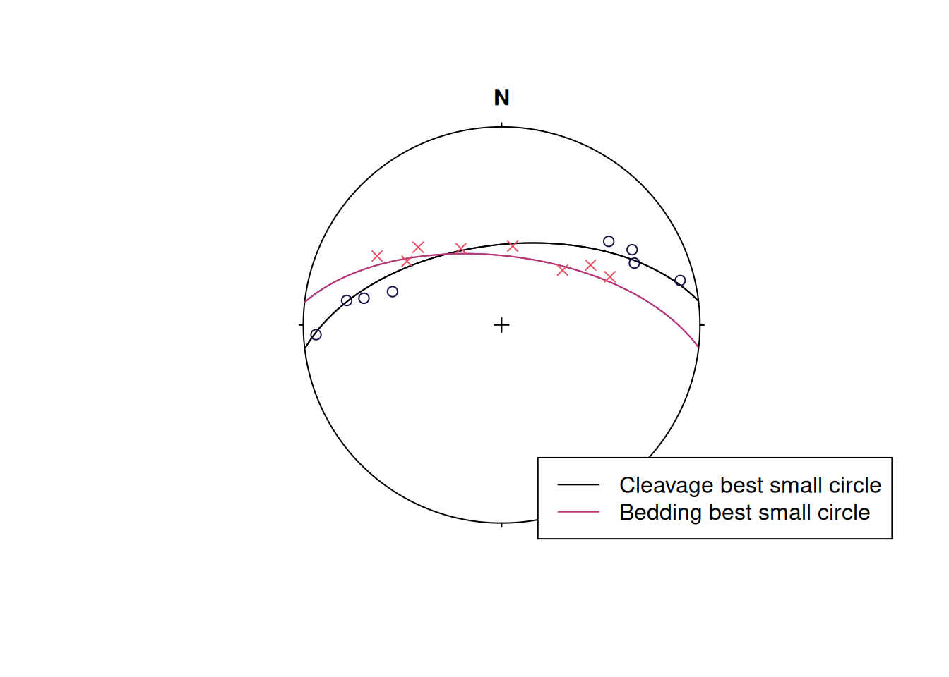
Summary
The regression was successful. The R2 values indicate a better fit for the cleavage, but a slightly poorer fit for the bedding. Hence, the poles to bedding seem to be aligned along a great circle, while the poles to cleavage better fit a small-circle arrangement.
Alternative
The Gray et al. (1980) algorithm is an alternative method for small- and great-circle fits using regression_smallcircle_gray() or regression_greatcircle_gray():
cleavage_sc2 <- regression_smallcircle_gray(cleavage)
bedding_sc2 <- regression_smallcircle_gray(bedding)

# Half-apical angle of small-circle cone (in degrees)
cleavage_sc2$cone
#> [1] 88.24055
bedding_sc2$cone
#> [1] 87.7376
regression_gray(x, out) is a convenience function where the out argument specifies the type of regression ("small" or "great" circle). If out = "both", the two solutions are compared by testing whether the small-circle solution fits better than the great-circle solution:
cleavage_sc3 <- regression_gray(cleavage, out = "both")
bedding_sc3 <- regression_gray(bedding, out = "both")

cleavage_sc3$comparison
#> $Vr
#> [1] 0.3612363
#>
#> $df1
#> [1] 1
#>
#> $df2
#> [1] 5
#>
#> $p_value
#> [1] 0.5740261
#>
#> $interpretation
#> [1] "no significant improvement over the great circle (p>=0.05)"
bedding_sc3$comparison
#> $Vr
#> [1] 0.09670531
#>
#> $df1
#> [1] 1
#>
#> $df2
#> [1] 5
#>
#> $p_value
#> [1] 0.7683665
#>
#> $interpretation
#> [1] "no significant improvement over the great circle (p>=0.05)"
References
Bachmann, F., Jupp, P. E., & Schaeben, H. (2014). Estimating the number and locations of Euler poles. International Journal on Geomathematics, 5(2), 289–301. https://doi.org/10.1007/s13137-014-0064-2
Davis, J. R., & Titus, S. J. (2017). Modern methods of analysis for three-dimensional orientational data. Journal of Structural Geology, 96, 65–89. https://doi.org/10.1016/j.jsg.2017.01.002
Gray, N. H., Geiser, P. A., & Geiser, J. R. (1980). On the least-squares fit of small and great circles to spherically projected orientation data. Journal of the International Association for Mathematical Geology, 12(3), 173–184. https://doi.org/10.1007/BF01091203
Ramsay, J. G. (1967). Folding and Fracturing of Rocks. McGraw-Hill.