Least-Squares Small and Great Circle Fit for Spherical Data

Finds the best small and great circles using the algorithm by Gray et al. (1980)

Usage

regression_gray(
  x,
  out = c("great", "small", "both"),
  sigma2 = 10,
  tol = NULL,
  max_iter = 100,
  verbose = FALSE
)

regression_smallcircle_gray(
  x,
  sigma2 = 10,
  tol = NULL,
  max_iter = 100,
  verbose = FALSE
)

regression_greatcircle_gray(
  x,
  sigma2 = 10,
  tol = NULL,
  max_iter = 100,
  verbose = FALSE
)

Arguments

x: object of class "Vec3", "Line", "Ray", or "Plane", where the rows are the observations and the columns are the coordinates.
out: character. Type of regression. "small" for a small-circle fit, "great" for the great-circle fit, and "both" for small- and great-circle estimates.
sigma2: numeric. Known error in degrees for a goodness-of-fit test. Default is 10
tol: numeric. Machine precision. Defaults to getOption("structr.tol").
max_iter: integer. Number of Newton-Lagrange optimizations. Default is 100
verbose: logical. Whether results of the iteration should be printed during the calculation. Default is FALSE

Value

list.

vec: Line of Vec3 object, sthe axis of the circle solution
cone: Half-apical angle of the small-circle in degrees. Alway 90° for a great-circle solution.
r_squared: Residual sum of squares
residuals: Per-point residuals
iterations, converged, p: Newton-iteration diagnostics
type: character. Type of the solution
statistic, df, p_value: Statistic, degrees of freedom and p-value of the $\chi^2$ goodness-of-fit test

If out = 'both, the a comparison of both solutions is added to the output:

V_r: Test statistic $V_r$
df1, df2: Degrees of freedom of the small and the great circle data, respectively
p_value: P-value of the comparison test

Details

Goodness-of-fit test

$\chi^2$ goodness-of-fit check against an independently known error variance $\sigma^2$ $$E(\sum R_i^2) = (p-q) \sigma^2$$, $q=3$ (great circle) or $q=4$ (small circle).

Test whether a small-circle fit is a significant improvement over the

corresponding great-circle fit

$$V_r = (p-3) [(r_g - r_c) / r_c] ~ F(1, p-3)$$ under the paper's normal-residual assumptions.

References

Gray, N.H., Geiser, P.A., Geiser, J.R. (1980). On the least-square fit of small and great circles to spherically projected data. Mathematical Geology, Vol. 12, No. 3, 1980.

Examples

data("gray_example")

# regression:
best_clea <- regression_gray(gray_example[1:8, ], out = "both")
best_bedd <- regression_gray(gray_example[9:16, ], out = "both")
best_all <- regression_gray(gray_example, out = "both")

# R-squared values:
best_clea$great$r_squared
#> [1] 0.0162995
best_bedd$great$r_squared
#> [1] 0.01157816
best_all$great$r_squared
#> [1] 0.1340548

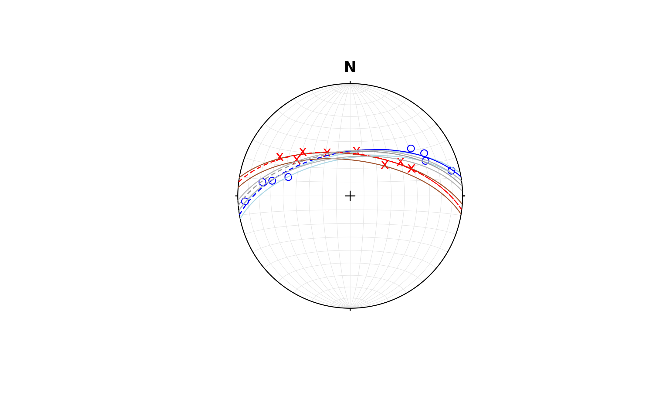
stereoplot()
points(gray_example[1:8, ], col = "blue")
points(gray_example[9:16, ], col = "red", pch = "x")

# best for cleavage
lines(best_clea$small$vec, best_clea$small$cone, col = "lightblue")
lines(best_clea$great$vec, 90, lty = 2, col = "blue")

# best for bedding
lines(best_bedd$small$vec, best_bedd$small$cone, col = "sienna")
lines(best_bedd$great$vec, 90, lty = 2, col = "red")

# best for all
lines(best_all$small$vec, best_bedd$small$cone, col = "gray70")
lines(best_all$great$vec, 90, lty = 2, col = "gray60")


# Compare small and great-circle solution:
regression_gray(gray_example[1:8, ], out = "both")$comparison
#> $Vr
#> [1] 0.3612363
#> 
#> $df1
#> [1] 1
#> 
#> $df2
#> [1] 5
#> 
#> $p_value
#> [1] 0.5740261
#> 
#> $interpretation
#> [1] "no significant improvement over the great circle (p>=0.05)"
#> 
regression_gray(gray_example[9:16, ], out = "both")$comparison
#> $Vr
#> [1] 0.09670531
#> 
#> $df1
#> [1] 1
#> 
#> $df2
#> [1] 5
#> 
#> $p_value
#> [1] 0.7683665
#> 
#> $interpretation
#> [1] "no significant improvement over the great circle (p>=0.05)"
#> 
regression_gray(gray_example, out = "both")$comparison
#> $Vr
#> [1] 0.04754425
#> 
#> $df1
#> [1] 1
#> 
#> $df2
#> [1] 13
#> 
#> $p_value
#> [1] 0.8307783
#> 
#> $interpretation
#> [1] "no significant improvement over the great circle (p>=0.05)"
#>