Strain and Vorticity Analysis

Tobias Stephan

2026-11-02

This tutorial demonstrates how to perform strain and vorticity analysis using the {structr} package in R.

library(structr)

Strain analysis

Import some $R_f/\phi$ data from elliptical strain markers:

data(ramsay)
head(ramsay)
#>         R   phi
#> [1,] 1.24 35.96
#> [2,] 1.52 27.59
#> [3,] 1.33 36.91
#> [4,] 1.78 27.31
#> [5,] 1.51 17.73
#> [6,] 1.70 24.45

The mean strain ellipse (shape and orientation) of deformed elliptical objects used as strain markers can be calculated from the mean shape matrix and its eigenvalues and eigenvectors¹:

ramsay_mean <- mean_strain_ellipse(r = ramsay[, 1], phi = ramsay[, 2])
print(ramsay_mean)
#> $R
#> [1] 1.628138
#> 
#> $phi
#> [1] 25.73632
#> 
#> $R_CI
#> [1] 1.59275 1.66359
#> 
#> $phi_CI
#> [1] 24.71905 26.75180

The {structr} algorithm also calculates bootstrapped 95% confidence intervals.

To visualize the distribution of the strain values, we can calculate densities in $R_f/\phi$ space² and plot them in an $R_f/\phi$ diagram³:

Rphi_plot(r = ramsay[, 1], phi = ramsay[, 2])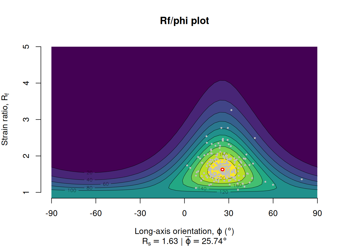

or in an equidistant polar plot⁴:

Rphi_polar_plot(ramsay[, 1], ramsay[, 2], proj = "eqd")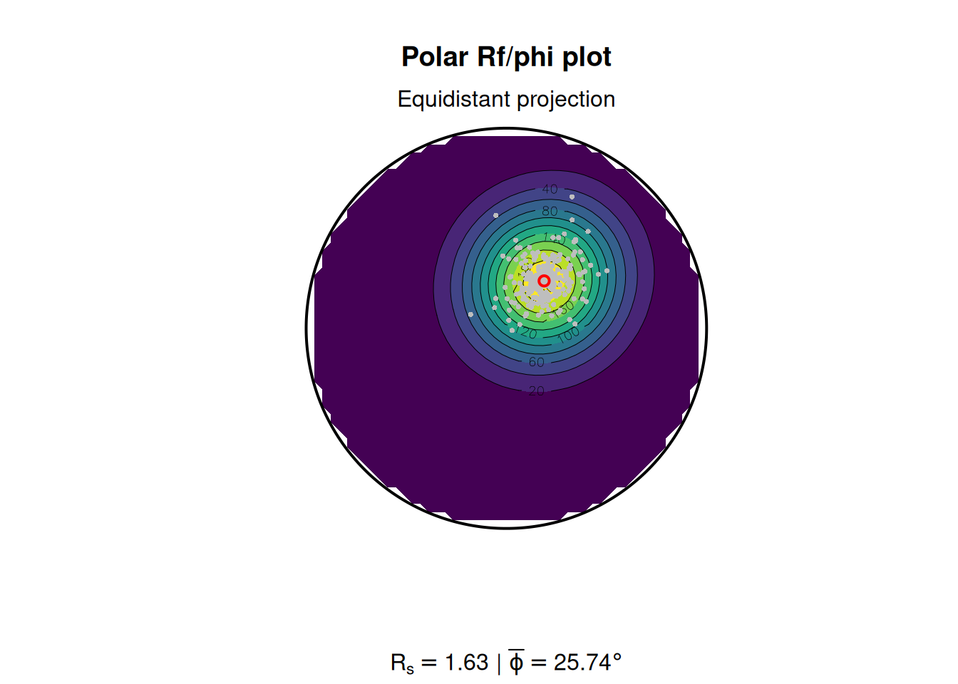

3D Strain

Three-dimensional strain data are expressed by the ratios of the magnitudes of the three principal axes of the strain ellipsoid, $X \geq Y \geq Z$. They can be represented in the Flinn diagram⁵, either linear or logarithmic:

data("holst")
R_XY <- holst[, "R_XY"]
R_YZ <- holst[, "R_YZ"]

flinn_plot(cbind(R_XY, R_YZ), log = TRUE, col = "#B63679", pch = 16)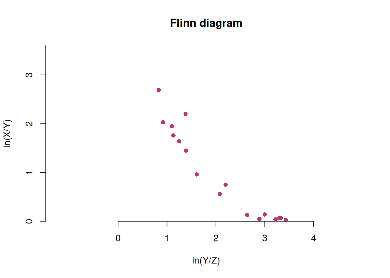

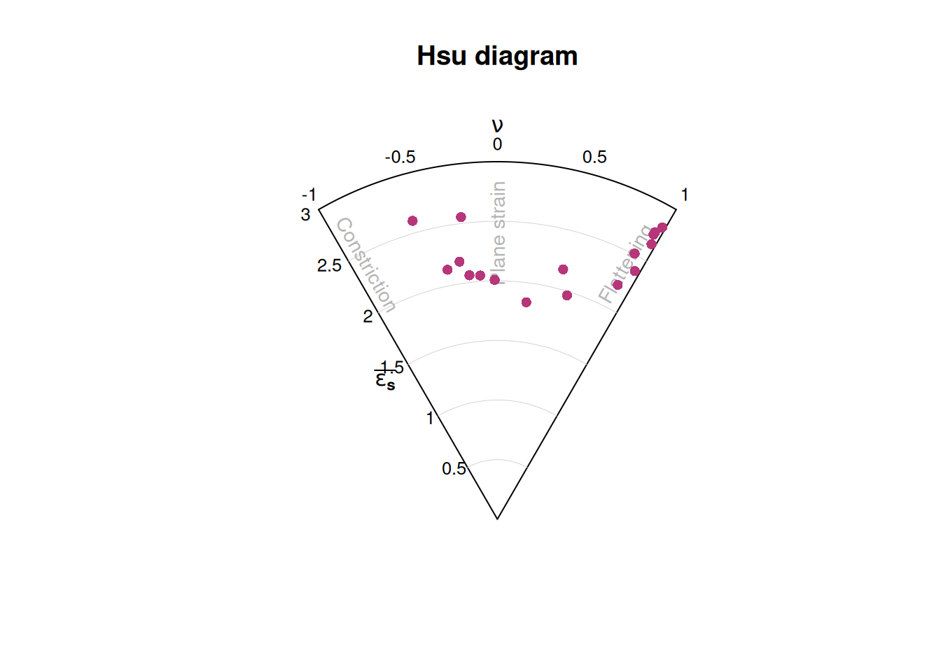
or in the Hsu diagram⁶ using the natural octahedral unit strain⁷ ($\bar{\epsilon}_s$) and the Lode parameter⁸ ($\nu$):

hsu_plot(cbind(R_XY, R_YZ), col = "#B63679", pch = 16)

Vorticity analysis

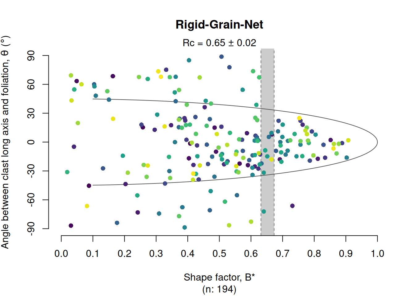
The Rigid Grain Net (Jessup et al., 2007)⁹ plots the aspect ratio (R) of porphyroclasts against their long-axis orientation with respect to the foliation (phi), on top of the theoretical fields of stable-sink and continuously rotating rigid clasts. The plot estimates the critical aspect ratio $R_c$ that marks the transition between clasts that reach a stable-sink position and clasts that rotate indefinitely. The mean kinematic vorticity number follows from this threshold as $W_m = (R_c^2 - 1)/(R_c^2 + 1)$. Uncertainties for $R_c$ are estimated using the bootstrap method described in Stephan et al. (2025)¹⁰.

data(shebandowan)
set.seed(20250411)

# Color code porphyroclasts by size of clast (area in log-scale):
RGN_plot(shebandowan$r, shebandowan$phi, col = assign_col(log(shebandowan$area)), pch = 16)