Simple fault analysis

The PT-techniques is a graphical solution of the Wallace-Bott hypothesis, i.e. fault slip occurs parallel to the maximum shear stress. It calculates PT-axes, kinematic planes (also movement planes), and the dihedra separation plane.

Usage

Fault_PT(x, ptangle = 90)

Arguments

x

"Fault" object where the rows are the observations, and the columns the coordinates. Object must be complete, i.e. no NA values. For Michael's, Angelier's, and Yamaji-Sato's methods, at least 4 rows of fault measurements are required, while Hansen's method requires at least 7.

ptangle

numeric. angle between P and T axes in degrees (90° by default).

Value

list. p and t are the P and T axes as "Line" objects, m and d are the M-planes and the dihedra separation planes as "Plane" objects

See also

Other stress-inversion: slip_inversion(), slip_inversion_angelier(), slip_inversion_hansen(), slip_inversion_hansen_boot(), slip_inversion_michael(), slip_inversion_simple(), slip_inversion_wissi(), slip_inversion_yamaji_sato()

Examples

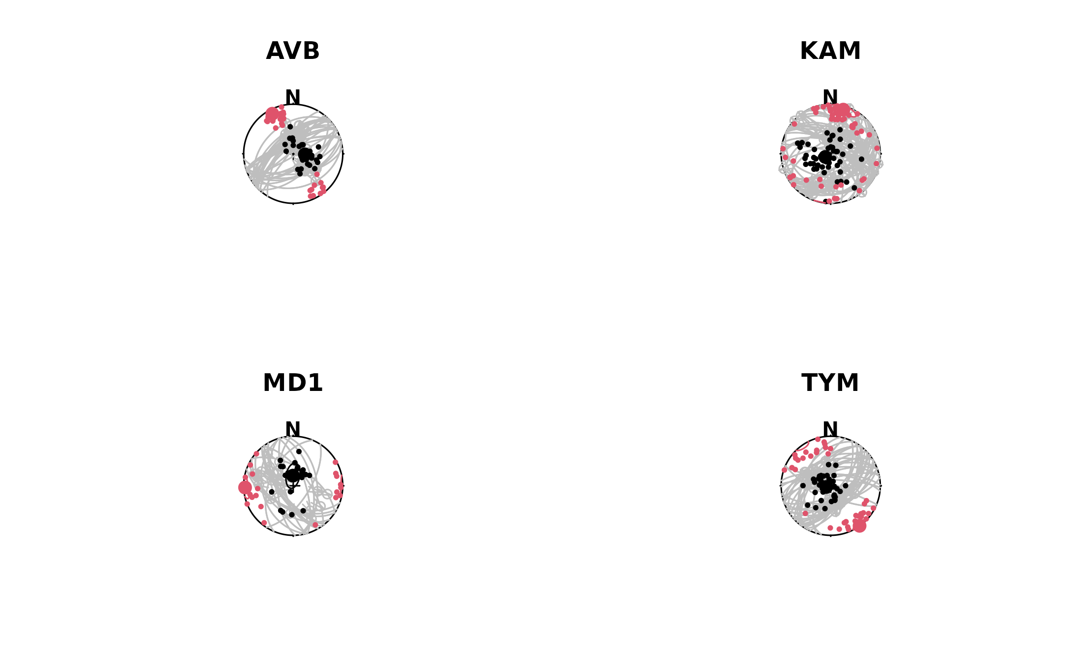
set.seed(20250411)

nx <- length(angelier1990)
par(mfrow = c(2, nx/2))

invisible(lapply(seq_len(nx), function(i) {
  # inversion
  x <- angelier1990[[i]]
  xpt <- Fault_PT(x)

  stereoplot(title = names(angelier1990)[i], guides = FALSE)
  angelier(x, col = "grey")
  points(xpt$p, pch = 16, cex = 0.6, col = 1)
  points(xpt$t, pch = 16, cex = 0.6, col = 2)
  stereo_confidence(xpt$p, pch = 16, cex = 1.5, col = 1, params = c(n_iter = 1e3))
  stereo_confidence(xpt$t, pch = 16, cex = 1.5, col = 2, params = c(n_iter = 1e3))
}))