Stress Inversion for Fault-Slip Data after Angelier (1990)

Direct inversion after the algorithm of Angelier (1990) with iterative refinement after Mostafa (2005)

Usage

slip_inversion_angelier(
  x,
  weights = NULL,
  max_iter = 100L,
  tol = 1e-06,
  n_psi = 361L,
  friction = 0.6,
  flip = FALSE
)

Arguments

x: "Fault" object where the rows are the observations, and the columns the coordinates. Must have at least 4 fault measurements.
weights: numeric. Weightings for the faults. Must have the same length as x
max_iter: integer. Maximum iteration count (default 50) for Mostafa (2005) optimization. Set to 0 for no optimization.
tol: numeric. Convergence tolerance on max absolute change in TR elements between iterations (default 1e-6)
n_psi: integer. Number of psi grid points for each step (default 361)
friction: numeric. Coefficient of friction (0.6 by default)
flip: logical. Flip if you want to have the negative stress tensor, i.e. sigma 1 and 3 will be flipped.

Value

a named list with the following components:

stress_tensor: "ellipsoid" object. Best-fit devitoric stress tensor in input coordinate frame
principal_axes: "Line" objects. Orientation of the principal stress axes as unit vectors (max to min)
tensor_params: the four tensor parameters (Eq. 4.87)
principal_vals: eigenvalues of the stress tensor ($\sigma_1 >= \sigma_2 >= \sigma_3$)
stress_shape: list Stress shape ratio. See stress_shape().
misfit: list. Misfit parameters. See slip_inversion_misfit().
SHmax: numeric. Direction of maximum horizontal stress (in degrees)
tau_mean: numeric. Average resolved shear stress on each plane. Should be close to 1.
stress_components: matrix. The resolved shear and normal stresses, the slip and dilation tendency on each plane. See tau2shearnorm() and tau2tendency().
n_iter: number of Mostafa iterations performed
method: character. The inversion method used, equal to method argument.

Details

The reduced stress tensor (Eq. 4.87) is parameterised as: $$T_R = \begin{bmatrix} \cos(\psi) & d & e \\ d & \cos(\psi+2\pi/3) & f \\ e & f & \cos(\psi + 4\pi/3) \end{bmatrix} $$ with two normalisation constraints (Pascal, 2022; Eqs 4.88–4.89):

$T_{11} + T_{22} + T_{33} = 0$ (deviator)
$T_{11}^2 + T_{22}^2 + T_{33}^2 = 3/2$ (fixes $\lambda = \sqrt(3)/2$)

The four unknowns are $\psi$, $d$, $e$, $f$.

Minimisation function (Eq. 4.101): $F_4 = \sum_i \upsilon_i^2$, where $\upsilon_i = \lambda * \hat{s}_i - \tau_i$

$dF_4/d(d,e,f)$ = 0 yields a 3x3 linear system in ($d$,$e$,$f$) given $\psi$. $dF_4/d\psi = 0$ is nonlinear; solved here by grid search + Brent refinement.

Mostafa (2005) replaces the global $\lambda$ with per-fault $\lambda_i$ equal to the shear traction magnitude on each plane and iterates until convergence.

Note

The solution can be refined iteratively by weighting the faults using the RUP values. This could be done using scale_weights() which scales the RUP values:

 # run a first inversion:
 first <- slip_inversion_angelier(x)
 first$

 # in the
 second <- slip_inversion_angelier(x, weights = scale_weights(first$misfit$rup, error_type = 'rup'))
 print(second)

References

Angelier, J. (1990). Inversion of field data in fault tectonics to obtain the regional stress—III. A new rapid direct inversion method by analytical means. Geophys. J. Int, 103, 363–376. https://doi.org/10.1111/j.1365-246X.1990.tb01777.x

Pascal, C. (2022). Paleostress Inversion Techniques. Chapter 4, Sections 4.2.3 and 4.2.4.

Mostafa, M. E. (2005). Iterative direct inversion: An exact complementary solution for inverting fault-slip data to obtain palaeostresses. Computers & Geosciences, 31(8), 1059–1070. https://doi.org/10.1016/j.cageo.2005.02.012

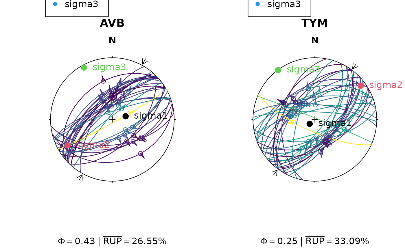
Examples

nx <- length(angelier1990)
par(mfrow = c(1, nx))

invisible(lapply(seq_len(nx), function(i) {
  # inversion
  x <- angelier1990[[i]]
  res <- slip_inversion_angelier(x, max_iter = 0)

  # some stress shape
  phi_val <- round(res$stress_shape$phi, 2)

  # misfit
  rup_val <- round(res$misfit$rup_mean, 2)

  # Plot the faults (color-coded by RUP%) and show the principal stress axes
  stereoplot(title = names(angelier1990)[i], guides = FALSE)
  stereo_shmax(res$SHmax)
  fault_plot(x, col = assign_col(res$misfit$rup))
  points(res$principal_axes, col = 1:3, pch = 16, cex = 1.5)
  text(res$principal_axes,
    label = rownames(res$principal_axes),
    col = 1:3, adj = -.25
  )
  legend("topleft", col = 2:4, legend = rownames(res$principal_axes), pch = 16)
  title(sub = bquote(Phi == .(phi_val) ~ "|" ~ bar("RUP") == .(rup_val) * "%"))
}))