Weighted Iterative Sigma-Space Inversion (WISSI)

Combines four classic fault slip inversion algorithms into a single coherent framework operating in the Yamaji-Sato 5-sphere sigma-space. Integrates the linear eigenvector approach of Yamaji & Sato (2006), the magnitude-aware upsilon criterion of Angelier (1990) and Mostafa (2005), the sense annealing strategy inspired by Hansen (2013), and the analytic uncertainty framework of Michael (1984), extended to the curved geometry of the 5-sphere.

Usage

slip_inversion_wissi(
  x,
  weights = NULL,
  sigma_alpha_deg = 10,
  gamma_max = 10,
  n_anneal = 8L,
  max_iter = 50L,
  tol_deg = 1e-04,
  run_stage4 = TRUE,
  robust = TRUE,
  robust_kernel = c("huber", "tukey", "andrews"),
  robust_k_deg = 30,
  robust_mad_k = 2.5,
  init_median = TRUE
)

Arguments

x

"Fault" object where the rows are the observations, and the columns the coordinates. Object must be complete, i.e. no NA values. For Michael's, Angelier's, and Yamaji-Sato's methods, at least 4 rows of fault measurements are required, while Hansen's method requires at least 7.

weights

Optional length-N numeric vector of non-negative data quality weights. NA values are replaced with the observed mean before scaling (neutral imputation). The vector is normalised internally so that mean(weights) = 1, meaning only the ratios between weights matter. Use scale_weights() to construct weights from field quality ranks, measurement errors, and prior RUP values. Default: uniform weights.

sigma_alpha_deg

Estimated angular measurement error of slip directions in degrees. Used in Stage 4 (analytic uncertainty) to scale the perturbation covariance matrix. A value of 10 ° is a conservative default for well-measured slickenlines; increase to 20-30 ° for less certain measurements. Default: 10.

gamma_max

Maximum sharpness parameter for the sense annealing schedule (Stage 3). Controls how strongly the final solution commits to the predicted slip sense. Higher values produce sharper sense discrimination; set to 0 to disable sense annealing entirely, making the inversion fully sense-agnostic in the style of Hansen (2013). Default: 10.

n_anneal

Number of annealing steps in the outer sense annealing loop (Stage 3). The sharpness parameter gamma increases linearly from 0 to gamma_max over n_anneal steps. More steps give a smoother transition between sense-agnostic and sense-committed behaviour. Default: 8.

max_iter

Maximum number of inner iterations per annealing step. Default: 50.

tol_deg

Convergence tolerance in angular stress distance (degrees). The inner loop terminates when the angular stress distance between successive iterates falls below this value. Because angular stress distance approximates the mean misfit angle (Yamaji & Sato 2006, Eq. 37), this tolerance has a direct physical interpretation. Default: 1e-4.

run_stage4

Logical. If TRUE, compute the analytic uncertainty estimates via eigenvalue perturbation theory (Stage 4) and return them in the unc element of the result. Setting to FALSE skips this step and is useful for bootstrap resampling where many inversions are performed. Default: TRUE.

robust

Logical. If TRUE, apply iteratively reweighted robust estimation using the kernel specified by robust_kernel. Faults with large angular misfits are progressively downweighted at each iteration, reducing the influence of outliers on the final tensor. Default: TRUE.

robust_kernel

Character string specifying the robust weighting kernel. One of:

"huber": Huber kernel: unit weight below the threshold robust_k_deg, declining as k/alpha above it. Gradual downweighting; the recommended default for most datasets.
"tukey": Tukey bisquare kernel: unit weight near zero misfit, declining smoothly to exactly zero at robust_k_deg. Faults beyond the threshold are completely excluded. Use when genuinely bad measurements are known to be present.
"andrews": Andrews sine kernel: similar to Tukey but differentiable at the threshold. Slightly smoother rejection profile.

Default: "huber".

robust_k_deg

Threshold angle in degrees for the robust kernel. Faults with angular misfit below this value receive full (or near-full) weight; faults above it are progressively downweighted or excluded depending on the chosen kernel. Should be set relative to the expected data noise level: 30° is appropriate for typical slickenline data, 20 ° for high-quality datasets, and 45 ° when significant scatter is expected. Default: 30.

robust_mad_k

Multiplier for the MAD-based outlier flagging applied after convergence. Faults whose angular misfit exceeds median(alpha) + robust_mad_k * 1.4826 * MAD(alpha) are reported in outliers_mad. This is a diagnostic flag only and does not affect the inversion result. Smaller values flag more faults; 2.5 corresponds roughly to the 99th percentile under a normal distribution. Default: 2.5.

init_median

Logical. If TRUE and robust = TRUE, initialise the iteration from the spatial median on S\(^5\) computed via the Weiszfeld algorithm, rather than the standard weighted eigenvector. The spatial median minimises the sum of angular stress distances to all single-fault solution poles and is substantially more resistant to outliers than the mean-based eigenvector initialisation. Has no effect when robust = FALSE. Default: TRUE.

Value

A named list with the following elements:

sigma: 3x3 reduced stress tensor in the input Cartesian frame.
y: 6D unit y-vector on \(S^5\) representing the optimal stress tensor.
sigma1, sigma2, sigma3: Unit vectors of the principal stress axes, from maximum (\(\sigma_1\)) to minimum (\(\sigma_3\)) compressive stress.
eigenvalues: Eigenvalues of sigma in decreasing order.
principal_axes: unit vectors of principal stress axes (max to min)
principal_vals: eigenvalues of stress_tensor (decreasing)
Phi: Shape ratio \(\Phi = (\sigma_1 - \sigma_2)/(\sigma_1 - \sigma_3) \in [0, 1]\).
alpha_deg: Per-fault unsigned angular misfit in degrees (0-90), the standard line metric.
alpha_signed_deg: Per-fault signed angular misfit in degrees (0-180). Values above 90 indicate that the recorded slip sense is opposite to the predicted shear traction direction.
mean_alpha: Mean unsigned angular misfit across all faults (degrees).
median_alpha: Median unsigned angular misfit (degrees). More robust than the mean in the presence of outliers.
suspected_flipped: Integer vector of row indices where alpha_signed_deg > 90, flagging faults whose recorded slip sense may be incorrect.
outliers_mad: Integer vector of row indices flagged as outliers by the MAD criterion (only when robust = TRUE).
n_flipped_sense: Number of faults whose slip sense was corrected internally during Stage 3.
slips_corrected: N x 3 matrix of sense-corrected slip vectors used in the final inversion.
mu: Per-fault magnitude weights \(\mu_i\) from Stage 2.
phi_sense: Per-fault \(\tanh\) sense confidence values from Stage 3. Positive values indicate consistent sense; negative values indicate corrected (flipped) senses.
w_robust: Per-fault robust kernel weights \(w_i^{\text{rob}}\) from the final iteration (only when robust = TRUE).
wt_combined: Per-fault combined weights \(\tilde{\omega}_i\) used in the final M5 matrix.
eigenvalue_gap: Difference \(\lambda_2 - \lambda_1\) of the final \(M_5\) matrix. Larger values indicate a better-conditioned solution.
M5_eigvals: All five eigenvalues of the final \(M_5\) matrix in decreasing order.
unc: List of analytic uncertainty estimates from Stage 4 (only when run_stage4 = TRUE), containing Cov5, Cov_y6, eigval_gap, cov_eigvals, sigma1_unc_deg, and Phi_unc.
n_iter_total: Total number of inner iterations performed across all annealing steps.

Details

Algorithm stages

WISSI proceeds through five sequential stages, each addressing a specific limitation of the classical inversion methods.

Stage 1 — Initialisation. Constructs the weighted moment matrix \(M_5 = \sum_i \omega_i \epsilon'_i \epsilon'^T_i\) in the 5D deviator subspace of the Yamaji-Sato sigma-space and returns its smallest-eigenvalue eigenvector as the initial stress estimate. When robust = TRUE and init_median = TRUE, the Weiszfeld algorithm on \(S^5\) is used instead, providing a starting point that is resistant to leverage points from badly oriented or erroneous fault data.

Stage 2 — Magnitude reweighting. Translates the Angelier (1990) and Mostafa (2005) upsilon (\(\upsilon_i\)) magnitude criterion into the sigma-space eigenproblem by replacing the global \(\lambda = \sqrt{3}/2\) with per-fault weights \(\mu_i = |\tau_i| / \lambda_{\max}\). Mechanically degenerate fault planes (those containing a principal stress axis, which produce near-zero shear traction) are automatically downweighted without requiring any explicit degeneracy test. Convergence is measured by the angular stress distance \(\Theta\) between successive iterates, which approximates the mean misfit angle (Yamaji & Sato 2006, Eq. 37) and therefore has a direct physical interpretation.

Stage 3 — Sense annealing. Replaces the binary majority-vote sense resolution of Yamaji & Sato (2006) with a continuous \(\tanh(\gamma \cdot \hat{\tau}_i \cdot \hat{s}_i)\) weighting schedule. At small \(\gamma\) (early annealing steps) the method is effectively sense-agnostic, as in Hansen (2013), providing robustness when slip senses are uncertain or partially incorrect. As \(\gamma\) increases toward gamma_max, the method commits progressively to the predicted slip sense, recovering the accuracy of Angelier (1990) for reliable data. Faults whose predicted and recorded senses are inconsistent have their slip vectors flipped internally; the number of such corrections is reported in n_flipped_sense.

Stage 4 — Analytic uncertainty. Propagates slip direction measurement noise (sigma_alpha_deg) through the eigenproblem via first-order perturbation theory, yielding a \(5 \times 5\) covariance matrix in sigma-space and approximate \(1\sigma\) confidence bounds on the principal stress axis orientations and \(\Phi\). This extends the analytic covariance framework of Michael (1984) to the geometrically correct curved space of the 5-sphere. The eigenvalue gap \(\lambda_2 - \lambda_1\) of \(M_5\) serves as a condition number: a small gap indicates that the solution is poorly separated from the next eigenvector and that uncertainty estimates may be unreliable.

Stage 5 (polyphase) — Spectral clustering. Available via slip_inversion_wissi_polyphase. Represents each fault by the pole of its solution great hypercircle on \(S^5\), builds a Gaussian affinity matrix using the angular stress distance \(\Theta\), and applies normalised spectral clustering with automatic phase count selection via the eigengap heuristic. WISSI is then run independently on each identified phase.

Robust estimation

When robust = TRUE, an additional misfit-based weight \(w_i^{\text{rob}} = \kappa(\alpha_i)\) is computed at each iteration and multiplied into the combined weight \(\tilde{\omega}_i = \omega_i \cdot \mu_i \cdot |\phi_i| \cdot w_i^{\text{rob}}\), where \(\alpha_i\) is the unsigned angular misfit between the predicted shear traction and the observed slip direction, \(\mu_i\) is the magnitude weight from Stage 2, and \(\phi_i\) is the sense confidence from Stage 3. The three available kernels \(\kappa\) differ in tail behaviour: the Huber kernel applies a gradual \(k/\alpha\) decay beyond the threshold and is the recommended default; the Tukey bisquare kernel hard-zeros faults beyond the threshold for aggressive rejection of confirmed bad measurements; the Andrews sine kernel provides a smooth differentiable alternative to Tukey. After convergence, faults are additionally screened using a median-absolute-deviation (MAD) criterion that adapts automatically to the noise level of the specific dataset, reported in outliers_mad. This flag is purely diagnostic and does not alter the inversion result.

References

Angelier, J. (1990). Inversion of field data in fault tectonics to obtain the regional stress. III. A new rapid direct inversion method by analytical means. Geophys. J. Int., 103, 363-376.

Hansen, J.A. (2013). Direct inversion of stress from sets of fault slip data with unknown slip sense. J. Struct. Geol., 51, 54-65.

Michael, A.J. (1984). Determination of stress from slip data: faults and folds. J. Geophys. Res., 89, 11517-11526.

Mostafa, M.E. (2005). Iterative linear inversion of stress tensor from fault-slip data. J. Struct. Geol., 27, 930-940.

Pascal, C. (2022). Paleostress Inversion Techniques. Elsevier.

Yamaji, A. & Sato, K. (2006). Distances for the solutions of stress tensor inversion in relation to misfit angles that accompany the solutions. Geophys. J. Int., 167, 933-942.

Stephan (in prep)

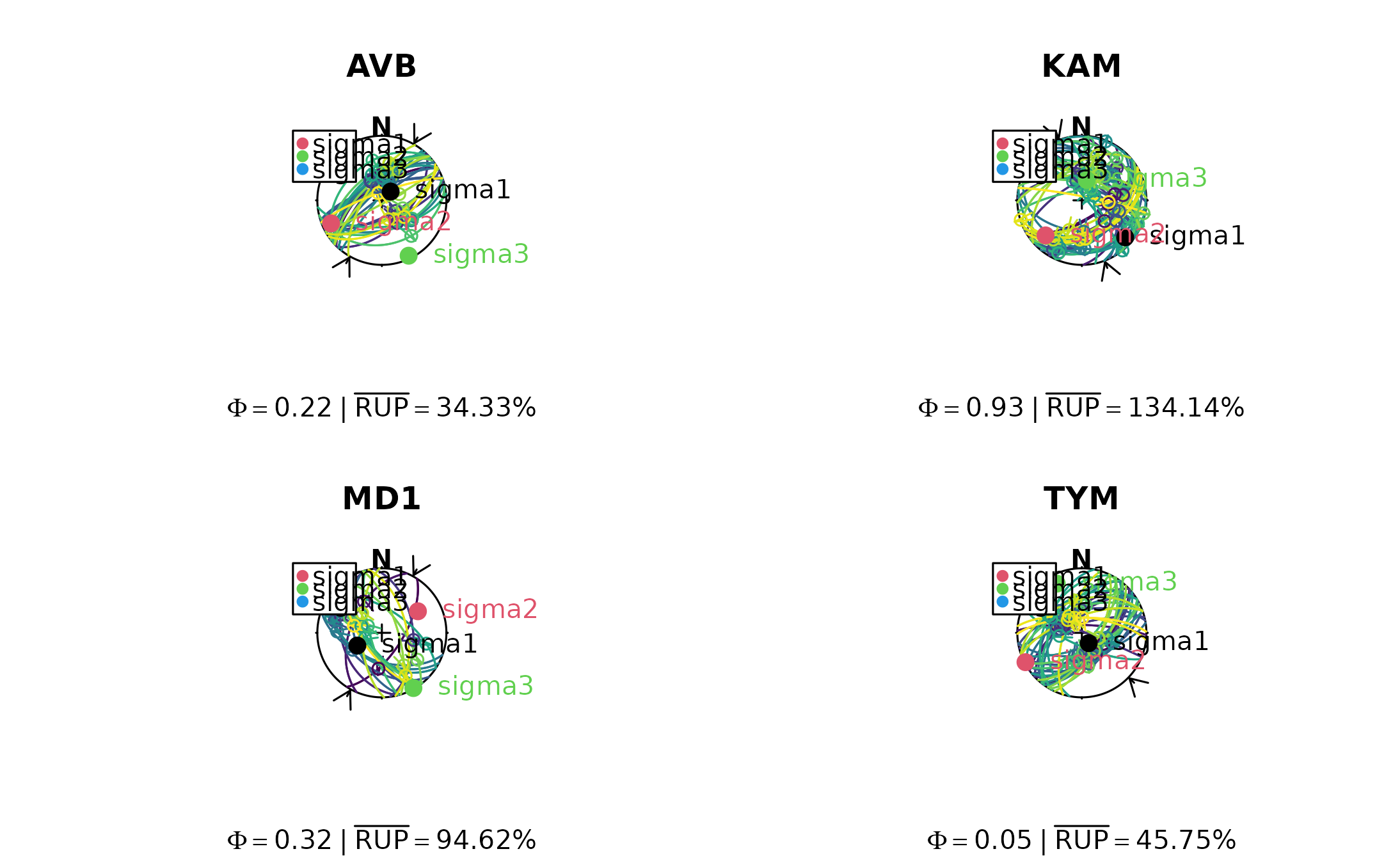
Examples

set.seed(20250411)

nx <- length(angelier1990)
par(mfrow = c(2, nx/2))

invisible(lapply(seq_len(nx), function(i) {
  # inversion
  x <- angelier1990[[i]]
  res <- slip_inversion_wissi(x)

  # some stress shape
  phi_val <- round(res$stress_shape$phi, 2)

  # misfit
  rup_val <- round(res$misfit$rup_mean, 2)

  # Plot the faults (color-coded by RUP%) and show the principal stress axes
  stereoplot(title = names(angelier1990)[i], guides = FALSE)
  stereo_shmax(res$SHmax)
  fault_plot(x, col = assign_col(res$misfit$rup))
  points(res$principal_axes, col = 1:3, pch = 16, cex = 1.5)
  text(res$principal_axes,
    label = rownames(res$principal_axes),
    col = 1:3, adj = -.25
  )
  legend("topleft", col = 2:4, legend = rownames(res$principal_axes), pch = 16)
  title(sub = bquote(Phi == .(phi_val) ~ "|" ~ bar("RUP") == .(rup_val) * "%"))
}))