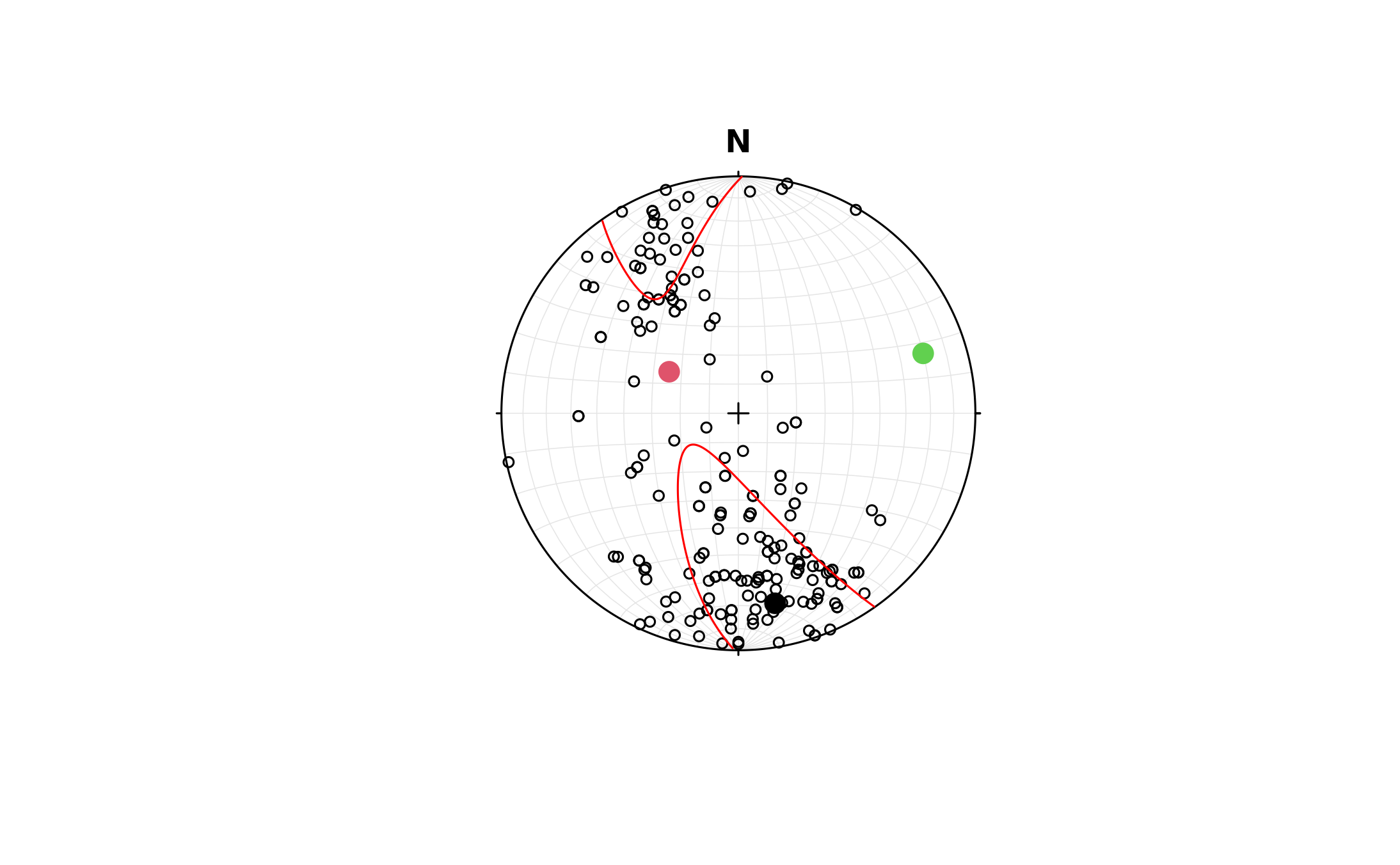
Confidence region for the mean of the Bingham distribution.

Confidence region for the mean of a Bingham distribution for anisotropic axial vectors. This function sometimes fails, if the data set is too concentrated, dispersed, or small? This is not a particularly high-quality implementation of the technique.

Usage

bingham_inference(x, n_points)

# S3 method for class 'Vec3'
bingham_inference(x, n_points = 0L)

# S3 method for class 'Line'
bingham_inference(x, n_points = 0)

# S3 method for class 'Plane'
bingham_inference(x, n_points = 0)

Arguments

x

object of class "Vec3", "Line", or "Plane", where the rows are the observations and the columns are the coordinates.

n_points

A real number (non-negative integer). If n_points > 0, then this function constructs a curve for the boundary of the 95% confidence region.

Value

A list with members directions, scatter, and angles. The first two members are identical to vectors and values in ot_eigen(). angles is a pair of real numbers. They describe the 95% confidence region, as two distances from the mean toward the two other principal dispersions, measured in radians along the unit sphere's surface. If the inference fails, then the angles are NA. If n_points > 0, then there is also a member points, which is a list of n_points + 1 lines delineating the confidence region.

See also

rbingham() for simulating a Bingham distribution, and bingham_MLE() to estimate distribution parameters.

Other distribution-inference: fisher-inference, watson-inference

Examples

r <- bingham_inference(example_planes, n_points = 1e3)
r$directions
#> Line object (n = 3):
#>        azimuth   plunge
#> [1,] 169.08091 19.46169
#> [2,] 300.98901 62.11934
#> [3,]  72.03016 19.15562

stereoplot()
points(example_planes, cex = 0.7)
points(r$directions, col = 1:3, pch = 16, cex = 1.5)
stereo_lines(r$points, col = 'red')