Maximum likelihood estimation of the Bingham distribution parameters.

MLE parameters of a Bingham distribution for anisotropic axial vectors. Uses a numerical integration (to compute the normalization constant) inside an numerical optimization (to maximize the likelihood). The Bingham probability density is proportional to \(\exp{(-x^T A x)}\), not \(\exp{(x^T A x)}\).

Usage

bingham_MLE(x, w, n_nonadapt, n_steps)

# S3 method for class 'Vec3'
bingham_MLE(x, w = NULL, n_nonadapt = 5L, n_steps = 1000L)

# S3 method for class 'Line'
bingham_MLE(x, w = NULL, n_nonadapt = 5L, n_steps = 1000L)

# S3 method for class 'Plane'
bingham_MLE(x, w = NULL, n_nonadapt = 5L, n_steps = 1000L)

Arguments

x

object of class "Vec3", "Line", or "Plane", where the rows are the observations and the columns are the coordinates.

w

optional weights for each observation in x. A vector of real numbers (non-negative), of length equal to x. They need not sum to 1; the function automatically normalizes them to do so.

n_nonadapt

A real number (non-negative integer). The number of refinements to use in the numerical integration. Note that each increment of n_nonadapt increases time and memory requirements by a factor of 4!

n_steps

A real number (positive integer). The number of steps to use in the numerical optimization.

Value

A list with members

A

symmetric 3x3 real matrix A,

values

a real 3D vector; the eigenvalues of A; sum to zero,

vectors

a rotation matrix; the eigenvectors of A are the columns,

error

integer; increase n_steps if error != 0, and

minEigenvalue

the minimum eigenvalue of the Hessian at the putative optimum; worry if this is not positive.

See also

bingham_inference() for confidence regions, and rbingham() to simulate a distribution.

Other distribution-MLE: dist.mle, fisher-mle, watson-mle

Examples

set.seed(2025041)
r <- bingham_MLE(example_planes)
print(r)
#> $error
#> [1] 0
#> 
#> $minEigenvalue
#> [1] 0.05781531
#> 
#> $A
#>            [,1]     [,2]       [,3]
#> [1,] -2.1069402 1.569431  0.9911088
#> [2,]  1.5694313 2.844694  1.3531322
#> [3,]  0.9911088 1.353132 -0.7377538
#> 
#> $values
#> [1] -2.766389 -1.081471  3.847860
#> 
#> $vectors
#> Line object (n = 3):
#>        azimuth   plunge
#> [1,] 169.08091 19.46169
#> [2,] 300.98901 62.11934
#> [3,]  72.03016 19.15562
#> 

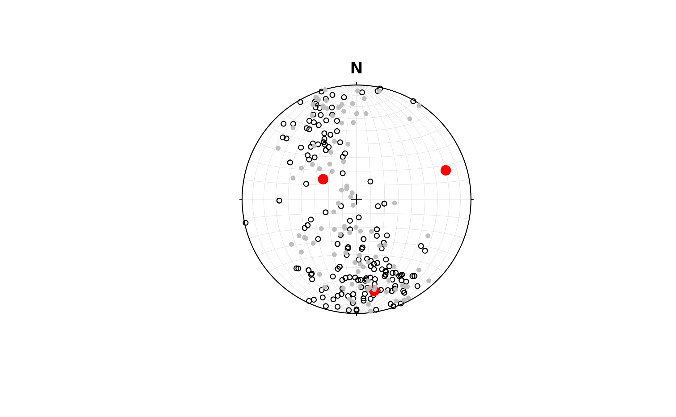
stereoplot()
points(example_planes, cex = 0.7)
points(r$vectors, col = 'red', pch = 16, cex = 1.5)

rnd <- rbingham(100, r$A, "Plane")
points(rnd, col = 'grey', cex = 0.7, pch = 16)