Maximum Likelihood Estimation of the Watson Distribution Parameters.

MLE parameters describing a Watson distribution for isotropic axial vectors. From Mardia and Jupp (2000, Section 10.3.2).

Usage

watson_MLE(x, shape)

# S3 method for class 'Vec3'
watson_MLE(x, shape = NULL)

# S3 method for class 'Line'
watson_MLE(x, shape = NULL)

# S3 method for class 'Plane'
watson_MLE(x, shape = NULL)

Arguments

x

object of class "Vec3", "Line", or "Plane", where the rows are the observations and the columns are the coordinates.

shape

NULL or character, either 'bipolar' or 'girdle'. If NULL, then this function chooses automatically.

Value

A list with members

muHat

a line, the MLE of the mean (identical to projected_mean() if x has a bipolar shape),

kappaHat

a real number, the MLE of the concentration,

shape

character, either 'bipolar' or 'girdle',

d3

a positive real number, the D3 from which kappaHat was computed, and

eigenvalues

(the eigenvalues of the \(\bar{T}\) matrix (orientation tensor), in descending order (see ot_eigen()).

See also

watson_inference() for confidence regions, and rwatson() to simulate a distribution.

Other distribution-MLE: bingham-mle, dist.mle, fisher-mle

Examples

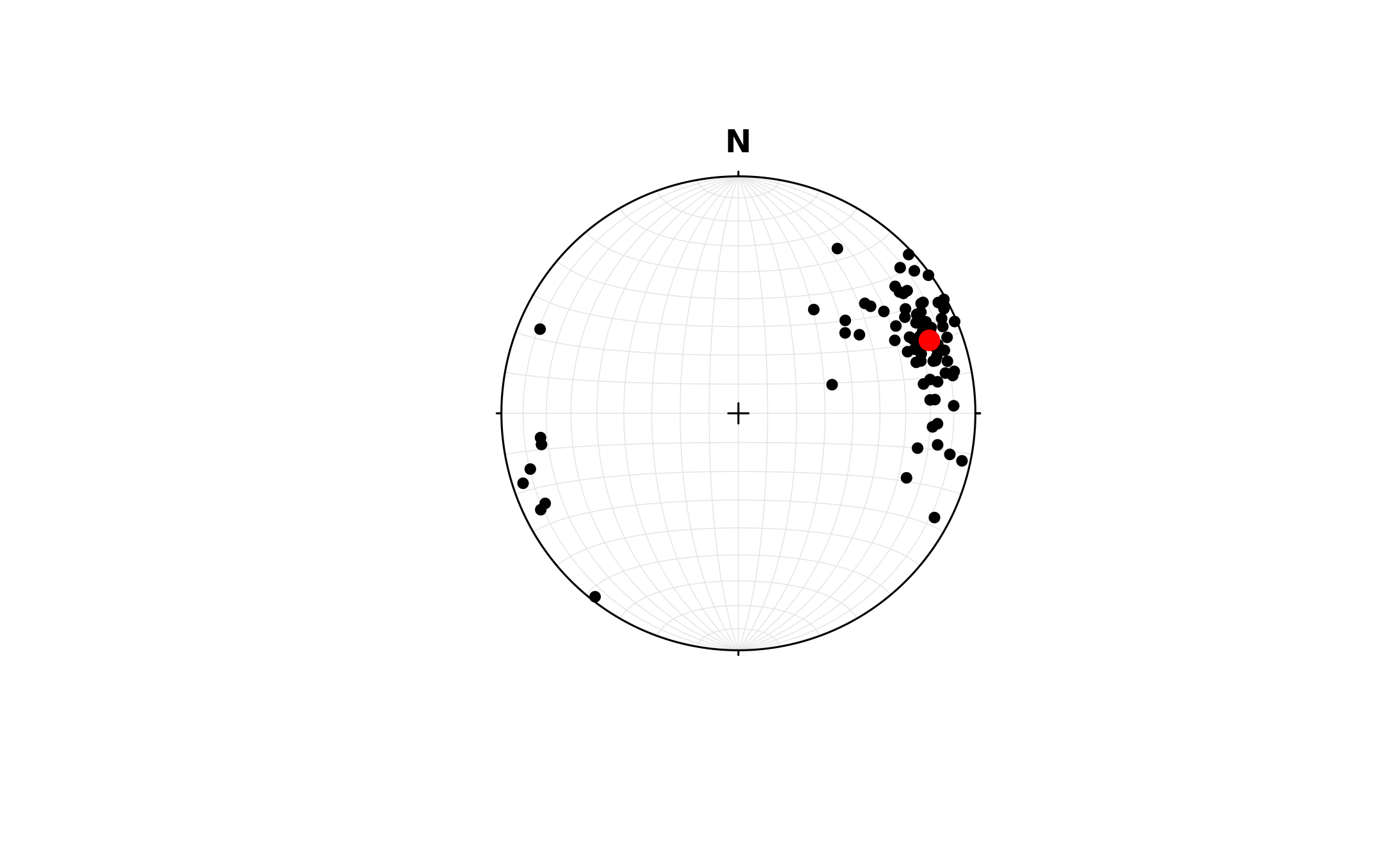
r <- watson_MLE(example_lines)
print(r)
#> $muHat
#> Line object (n = 1):
#>  azimuth   plunge 
#> 69.09796 14.82125 
#> 
#> $kappaHat
#> [1] 9.815405
#> 
#> $shape
#> [1] "bipolar"
#> 
#> $d3
#> [1] 0.8904488
#> 
#> $eigenvalues
#> [1] 0.89044880 0.06736731 0.04218389
#> 

plot(example_lines)
points(r$muHat, col = 'red', pch = 16, cex = 1.5)