Confidence Region for the Fisher Distribution Mean.

Confidence Region for the Fisher Distribution Mean.

Usage

fisher_inference(x, alpha)

# S3 method for class 'Vec3'
fisher_inference(x, alpha = 0.05)

# S3 method for class 'Ray'
fisher_inference(x, alpha = 0.05)

# S3 method for class 'Line'
fisher_inference(x, alpha = 0.05)

# S3 method for class 'Plane'
fisher_inference(x, alpha = 0.05)

Source

modified after geologyGeometry by Davis, J.R.

Arguments

x

object of class "Vec3", "Ray", or "Plane", where the rows are the observations and the columns are the coordinates.

alpha

A real number, between 0 and 1. The significance level for the confidence region.

Value

A list with members

muHat

a ray, identical to sph_mean()). The mean vector of the distribution.

kappaHat

a non-negative real number). The concentration parameter.

angle

a real number in [0, pi]). angle is the radius of the confidence region, measured along the surface of the sphere. In radians if x is a Vec3 class, in degrees otherwise.

#'

Details

Experiments with Fisher-distributed data sets suggest that the sample size n doesn't affect the accuracy much. kappa == 1 is too dispersed, but kappa == 3 is fine.

References

Tauxe (2010, p. 214). L. Tauxe 2010. Essentials of Paleomagnetism. xvi + 489 pp. Berkeley: University of California Press.

See also

rvmf() for simulating a von Mises-Fisher distribution, and fisher_MLE() to estimate distribution parameters.

Other distribution-inference: bingham-inference, watson-inference

Examples

set.seed(20250411)
x <- rvmf(100, mu = Ray(120, 50), k = 5)
r <- fisher_inference(x)
print(r)
#> $muHat
#> Ray object (n = 1):
#>   azimuth    plunge 
#> 118.32579  50.88713 
#> 
#> $kappaHat
#> [1] 4.952381
#> 
#> $angle
#> [1] 7.103673
#> 

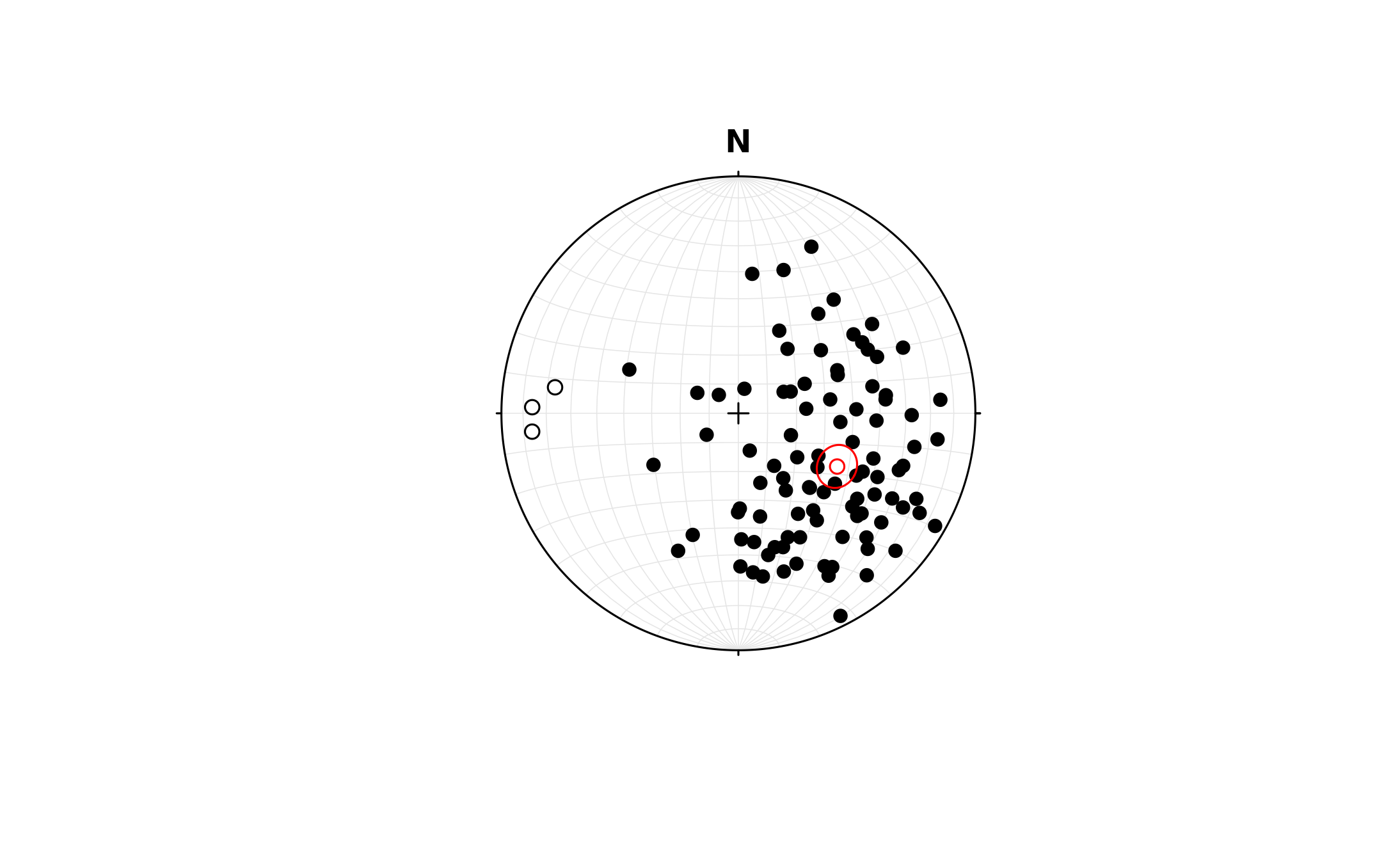
plot(x)
points(r$muHat, col = 'red')
lines(r$muHat, ang = r$angle, col = 'red')