6. Faults and Paleostress

Tobias Stephan

2025-10-28

This tutorial demonstrates the "Fault" object. It also shows how you can extract paleo-stress directions from fault slip data, and how you can derive displacement components from fault slip.

Fault objects

A fault is given by the orientation of its plane (dip direction and dip angle), the orientation of the slip (e.g. measured from striae, given in azimuth and plunge angles), and the sense of displacement:

my_fault <- Fault(120, 50, 60, 110, sense = -1)

Sense of fault displacement is 1 or -1 for normal or thrust offset, respectively.

Rake of the fault, i.e. the angle between fault slip vector and fault strike:

Fault_rake(my_fault)

## [1] -107.2294

Define a fault by just knowing the orientation of the fault plane, the sense, and the rake

# 1. Define a plane through dip direction, dip angle
fault_plane <- Plane(c(120, 120, 100), c(60, 60, 50)) 

# 2. Define a fault through the plane and rake angle:
Fault_from_rake(fault_plane, rake = c(84.7202, -10, 30))

## Fault object (n = 3):
##      dip_direction dip   azimuth    plunge sense
## [1,]           120  60 109.52858 59.581591     1
## [2,]           120  60 204.96163  8.649165    -1
## [3,]           100  50  30.36057 22.521012     1

Often, measured orientation angles can be (slightly) imprecise and subjected to some random noise. Thus the slip vector will not lie (perfectly) on the fault plane, judging by the measurements. To correct the measurements so that this will not be the case:

p <- Pair(120, 60, 110, 58)

misfit_pair(p)

## $fvec
## Vector (Vec3) object (n = 1):
##          x          y          z 
##  0.4306074 -0.7432627  0.5119940 
## 
## $lvec
## Vector (Vec3) object (n = 1):
##          x          y          z 
## -0.1752467  0.4876291  0.8552815 
## 
## $misfit
## [1] 0.02793105

correct_pair(p)

## Pair object (n = 1):
## dip_direction           dip       azimuth        plunge 
##     120.08575      59.20326     109.76769      58.79085

A "Pair" object is a container of associated plane and line measurements. Basically like a fault wihtout the sense of displacement.

Fault stress analysis

The Wallace-Bott hypothesis states that fault slip occurs parallel to the maximum shear stress. This allows to reconstruct stress axes using fault-slip data. {structr} offers several techniques to calculate the orientation of principal stress axes, the simple P-T method, and a fault-slip inversion technique.

P-T method

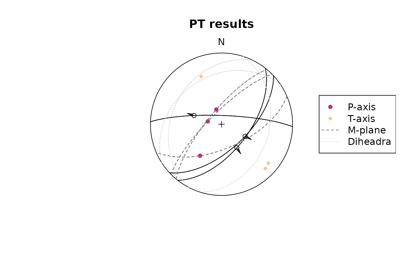
This simple technique calculates PT-axes, kinematic plane (M), and dihedra separation plane (d).

First we load some example data (here the first three faults from the TYM dataset by from Angelier, 1990)¹

data("angelier1990")
my_fault2 <- angelier1990$TYM[1:3, ]

print(my_fault2)

## Fault object (n = 3):
##      dip_direction dip  azimuth   plunge sense
## [1,]           137  61 117.0135 59.46650     1
## [2,]           128  59 146.8990 57.58045     1
## [3,]             2  80 287.5304 56.63295     1

my_fault2_PT <- Fault_PT(my_fault2)
print(my_fault2_PT)

## $p
## Line object (n = 3):
##       azimuth   plunge
## [1,] 340.6153 72.15071
## [2,] 281.6092 73.96385
## [3,] 214.3217 45.50717
## 
## $t
## Line object (n = 3):
##       azimuth   plunge
## [1,] 129.6815 15.44075
## [2,] 135.2532 13.45689
## [3,] 336.9158 27.88916
## 
## $m
## Plane object (n = 3):
##      dip_direction      dip
## [1,]      42.11395 81.26433
## [2,]     223.18909 81.43997
## [3,]     265.80721 58.54232
## 
## $d
## Plane object (n = 3):
##      dip_direction      dip
## [1,]      297.0135 30.53350
## [2,]      326.8990 32.41955
## [3,]      107.5304 33.36705

Plot the results

stereoplot(title = "PT results", guides = FALSE)
fault_plot(my_fault2)
points(my_fault2_PT$p, col = "#B63679FF", pch = 16)
points(my_fault2_PT$t, col = "#FEC287FF", pch = 18)
lines(my_fault2_PT$t, lty = 2, col = "grey40")
lines(my_fault2_PT$d, lty = 3, col = "grey80")

legend("right",
  legend = c("P-axis", "T-axis", "M-plane", "Diheadra"),
  col = c("#B63679FF", "#FEC287FF", "grey40", "grey80"),
  pch = c(16, 18, NA, NA), lty = c(NA, NA, 2, 3)
)

Fault slip inversion

Our goal is to find the single uniform stress tensor that most likely caused the faulting events. With only slip data to constrain the stress tensor the isotropic component can not be determined, unless assumptions about the fracture criterion are made. Hence inversion will be for the deviatoric stress tensor only. A single fault can not completely constrain the deviatoric stress tensor a, therefore it is necessary to simultaneously solve for a number of faults, so that a single a that best satisfies all of the faults is found.

This is equivalent to assuming that the stress field is a constant tensor within the region being studied for the duration of the faulting event.

{structr} provides a numerical solution to determine the orientation of the principal stresses from fault slip data using the Michael (1984) method². It uses bootstrapping for confidence intervals of the stress estimates.

First we load some example data (here the data from Angelier, 1990)³

test_data <- angelier1990$TYM

stereoplot(title = "Test data", guides = FALSE)
fault_plot(test_data, col = "grey30")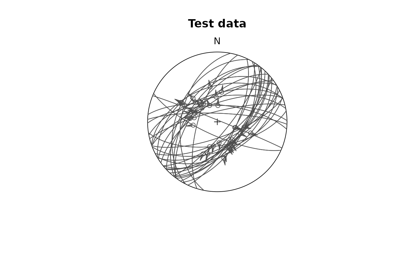

The stress inversion with 10 bootstraps:

test_res <- slip_inversion(test_data, boot = 10)

# Average beta angle
test_res$beta

## [1] 15.16869

# Average resolved shear stress
test_res$sigma_s

## [1] 0.9289024

To check the accuracy of the solution, you can evaluate

• the average angle β between the tangential traction predicted by the best stress tensor and the slip vector on each plane (ideally close to 0), and
• the average resolved shear stress on each plane (should be close to 1).

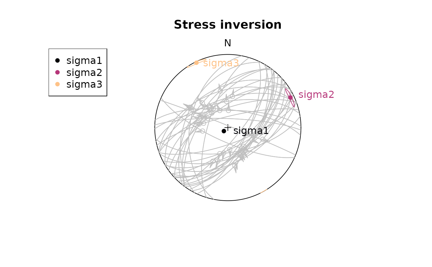
To visualizing the orientation of the principal stresses and the confidence region of the axes, you may use the stereoplot() functions from {structr}

cols <- c('#000004FF', "#B63679FF", "#FEC287FF")

stereoplot(title = "Stress inversion", guides = FALSE)
fault_plot(test_data, col = 'grey75')
stereo_confidence(test_res$principal_axes_conf$sigma1, col = cols[1])
stereo_confidence(test_res$principal_axes_conf$sigma2, col = cols[2])
stereo_confidence(test_res$principal_axes_conf$sigma3, col = cols[3])
text(test_res$principal_axes, 
     label = rownames(test_res$principal_axes), 
     col = cols, adj = -.25)
legend("topleft", col = cols, 
       legend = rownames(test_res$principal_axes), pch = 16)

The stress shape ratio Φ (Angelier 1979)⁴

test_res$phi

## [1] 0.101247

# 95% confidence interval
test_res$phi_conf

## [1] 0.07111952 0.12989809
## attr(,"conf.level")
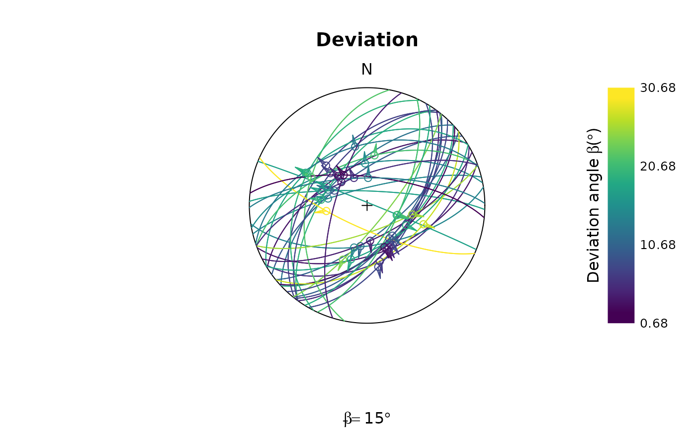
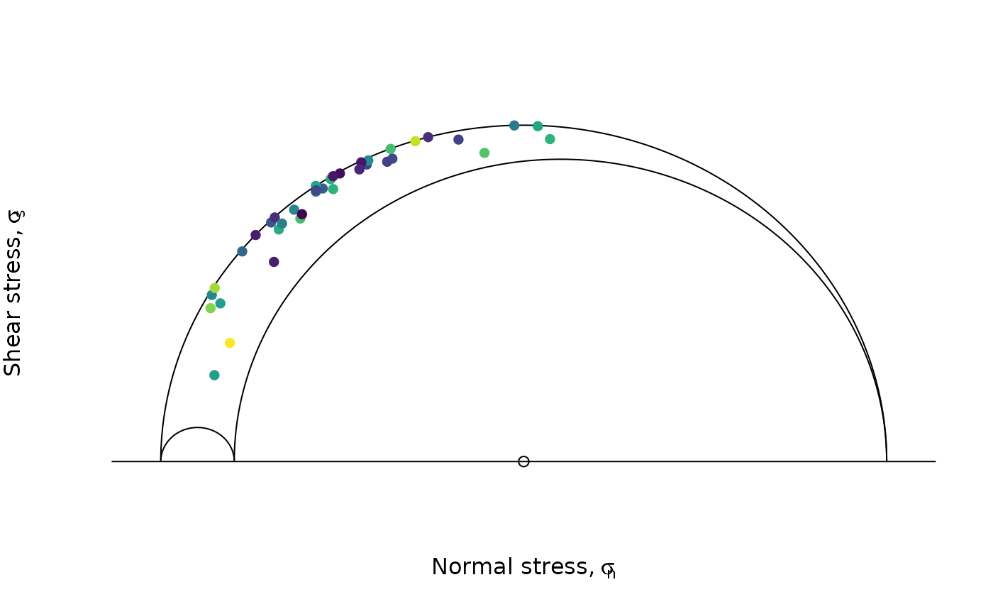
## [1] 0.95

The angle β is the angle between the tangential traction predicted by the best stress tensor and the slip vector. This deviation can be visualized in the stereoplot:

beta <- test_res$fault_data$beta

stereoplot(
  title = "Deviation", 
  sub = bquote(bar(beta) == .(round(test_res$beta)) * degree), 
  guides = FALSE)

fault_plot(test_data, col = assign_col(beta))
legend_c(
  seq(min(beta), max(beta), 10), 
  title = bquote("Deviation angle" ~ beta ~ "("*degree*")")
  )

Maximum horizontal stress⁵

We de fine a vertical plane in the geographic coordinate system, $\mathbb{G}$, using its unit normal vector, $\vec{n}^T_\mathbb{G} = (n_N, n_E, n_D) = (\cos\alpha, \sin\alpha, 0)$, where $\alpha$ is the normal’s trend angle measured clockwise from north and the plane’s strike is $\alpha+\pi/2$. We represent $\vec{n}$ with respect to the principal stress coordinate system using the transformation matrix

$$\begin{equation} \mathsf{A}_{\mathbb{S}\mathbb{G}} = \begin{pmatrix} \vec{\sigma}_1 \vec{g}_1 & \vec{\sigma}_1 \vec{g}_2 & \vec{\sigma}_1 \vec{g}_3 \\ \vec{\sigma}_2 \vec{g}_1 & \vec{\sigma}_2 \vec{g}_2 & \vec{\sigma}_2 \vec{g}_3 \\ \vec{\sigma}_3 \vec{g}_1 & \vec{\sigma}_3 \vec{g}_2 & \vec{\sigma}_3 \vec{g}_3 \\ \end{pmatrix} \end{equation}$$

(i.e. $a_{ij} = \sigma_i g_j$). Here $\sigma_i = (\sigma_{iN}, \sigma_{iE}, \sigma_{iD})$ are unit vectors in the principal stress directions (principal stress coordinate system $\mathbb{S}$ with unit vectors $\{ \mathbf{\vec{\sigma_1}}, \mathbf{\vec{\sigma_2}}, \mathbf{\vec{\sigma_3}} \}$) with respect to the geographic coordinate system ($\mathbb{G}$), and $\vec{g_1} = (1,0,0)$, $\vec{g_2} =(0,1,0)$ and $\vec{g_3} = (0,0,1)$ are the basis vectors in the geographic coordinate system. The normal vector expressed with respect to the principal stress system is then

$$\begin{equation} \vec{\mathbf{n}}_\mathbb{S} = \mathsf{A}_{\mathbb{S}\mathbb{G}}\vec{\mathbf{n}}_\mathbb{G} = \begin{pmatrix} \sigma_{1N}n_N + \sigma_{1E}n_E\\ \sigma_{2N}n_N + \sigma_{2E}n_E\\ \sigma_{3N}n_N + \sigma_{3E}n_E \end{pmatrix}, \end{equation}$$

where, for example, $\sigma_{1N}$ is the north component of the $\vec{\sigma}_1$ unit vector. In the principal coordinate system, the stress tensor is diagonal

$$\begin{equation} \mathsf{S}_\mathbb{S} = \begin{pmatrix} \lVert \sigma_1 \rVert & 0 & 0 \\ 0 & \lVert\sigma_2\rVert & 0 \\ 0 & 0 & \lVert\sigma_3\rVert \end{pmatrix} \end{equation}$$

and the normal stress acting on the vertical plane of interest is

$$\begin{equation} \begin{split} \sigma_n &= \left( \mathbf{\vec{n}}^T_\mathbb{S} \mathsf{S}_\mathbb{S} \mathbf{\vec{n}}_\mathbb{S} \right)\\ &= \left[ \lVert\sigma_1\rVert ( \sigma_{1N}n_N + \sigma_{1E}n_E )^2 + \lVert\sigma_2\rVert ( \sigma_{2N}n_N + \sigma_{2E}n_E )^2 + \lVert\sigma_3\rVert (\sigma_{3N}n_N + \sigma_{3E}n_E)^2 \right] \mathbf{\vec{n}}_{\mathbb{S}}\\ &= \lVert\sigma_n\rVert \mathbf{\vec{n}}_\mathbb{S}. \end{split} \end{equation}$$

This normal stress corresponds to the horizontal stress in the direction of $\mathbf{\vec{n}}$.

We can find the direction of the maximum horizontal stress analytically by differentiating the last equation with respect to $\alpha$.

$$\begin{equation} \frac{d\sigma_n}{d\alpha} = \left[ \lVert\sigma_1\rVert ( \sigma_{1E}^2 - \sigma_{1N}^2 ) + \lVert\sigma_2\rVert ( \sigma_{2E}^2 - \sigma_{2N}^2 ) + \lVert\sigma_3\rVert ( \sigma_{3E}^2 - \sigma_{3N}^2 ) \right] \sin{2\alpha} + 2 \left[\lVert\sigma_1\rVert \sigma_{1N} \sigma_{1E} + \lVert\sigma_2\rVert \sigma_{2N} \sigma_{2E} + \lVert\sigma_3\rVert \sigma_{3N} \sigma_{3E} \right] \cos{2\alpha}. \end{equation}$$

Table 1 Summary of the conditions under which the denominator of eq. (11) equals zero. $\alpha_H$ and $\alpha_1$ denote the trends of the axis of maximum horizontal stress, $\sigma_H$, and the principal axis of maximum compressive stress, $\mathbf{\vec{\sigma_1}}$, respectively.

Condition	Interpretation
$\sigma_{1N} = \pm \sigma_{1E}$ and $R = 1$	$\mathbb{S}_H$ undefined if $\mathbf{\vec{\sigma_1}}$ vertical, else $\alpha_H = \alpha_1$ (45$^{\circ}$ or 135°)
$\sigma_{1N} = \pm \sigma_{1E}$ and $\sigma_{2N} = \pm \sigma_{2E}$	$\mathbb{S}_H$ undefined if $R = 0$, else $\alpha_H = \alpha_1$ (45$^{\circ}$ or 135°)
$(\sigma_{1N}^2 - \sigma_{1E}^2) + (1 - R)(\sigma_{2N}^2 - \sigma_{2E}^2) = 0$	$\mathbb{S}_H$ undefined if $R = 0$, else $\alpha_H = \alpha_1$ (45$^{\circ}$ or 135°)

In general (cf. Table 1), $\sigma_n$ has one maximum and one minimum in the interval $0 \leq \alpha \leq \pi$ and setting the derivative in the last equation to zero, we find these stationary points:

$$\begin{equation} \tan{2\alpha} = \frac{ 2 ( \lVert\sigma_1\rVert \sigma_{1N} \sigma_{1E} + \lVert\sigma_2\rVert \sigma_{2N} \sigma_{2E} + \lVert\sigma_3\rVert \sigma_{3N} \sigma_{3E} )}{\lVert\sigma_1\rVert ( \sigma_{1E}^2 - \sigma_{1N}^2 ) + \lVert\sigma_2\rVert ( \sigma_{2E}^2 - \sigma_{2N}^2 ) + \lVert\sigma_3\rVert ( \sigma_{3E}^2 - \sigma_{3N}^2 )}. \end{equation}$$

Using the second derivative of $\sigma_n$ with respect to $\alpha$ we can determine whether $\sigma_n (\alpha)$ yields a maximum or a minimum value, and identify the $\sigma_H$ trend ($\alpha_H$) accordingly:

$$\begin{equation} \alpha_H = \begin{cases} \alpha & \text{if $\lVert\sigma_n (\alpha)\rVert$ is a maximum} \\ \alpha + \pi/2 & \text{if $\lVert\sigma_n (\alpha)\rVert$ is a minimum} \end{cases}. \end{equation}$$

Code

Define the orientation of the principle stress axes:

S1 <- Line(250.89, 70.07)
S3 <- Line(103.01, 17.07)

To get S2 - which is perpendicular to S1 and S3, we calculate the cross-product of the two vectors:

S2 <- crossprod(S3, S1)

The azimuth of SHmax for a given stress ratio R = 1:

SH(S1, S2, S3, R = 1) # in degrees

## [1] 70.89

For a several stress ratios:

R <- seq(0, 1, .1)
cbind(R, SH = SH(S1, S2, S3, R = R))

##         R       SH
##  [1,] 0.0 13.01021
##  [2,] 0.1 13.37695
##  [3,] 0.2 13.84162
##  [4,] 0.3 14.44908
##  [5,] 0.4 15.27621
##  [6,] 0.5 16.46586
##  [7,] 0.6 18.31445
##  [8,] 0.7 21.53704
##  [9,] 0.8 28.23884
## [10,] 0.9 45.01043
## [11,] 1.0 70.89000

And the SHmax for the slip inversion result from above:

SH(
  S1 = test_res$principal_axes[1, ], 
  S2 = test_res$principal_axes[2, ], 
  S3 = test_res$principal_axes[3, ],
  R = test_res$R)

## [1] 60.80844

Fault offsets

The offset along a fault can be factorized into several components.

Fig. 1: Graphic illustration of displacement components along a fault. $\mathbb{G}$ as the georeference frame with D = down, E = East, N = North.

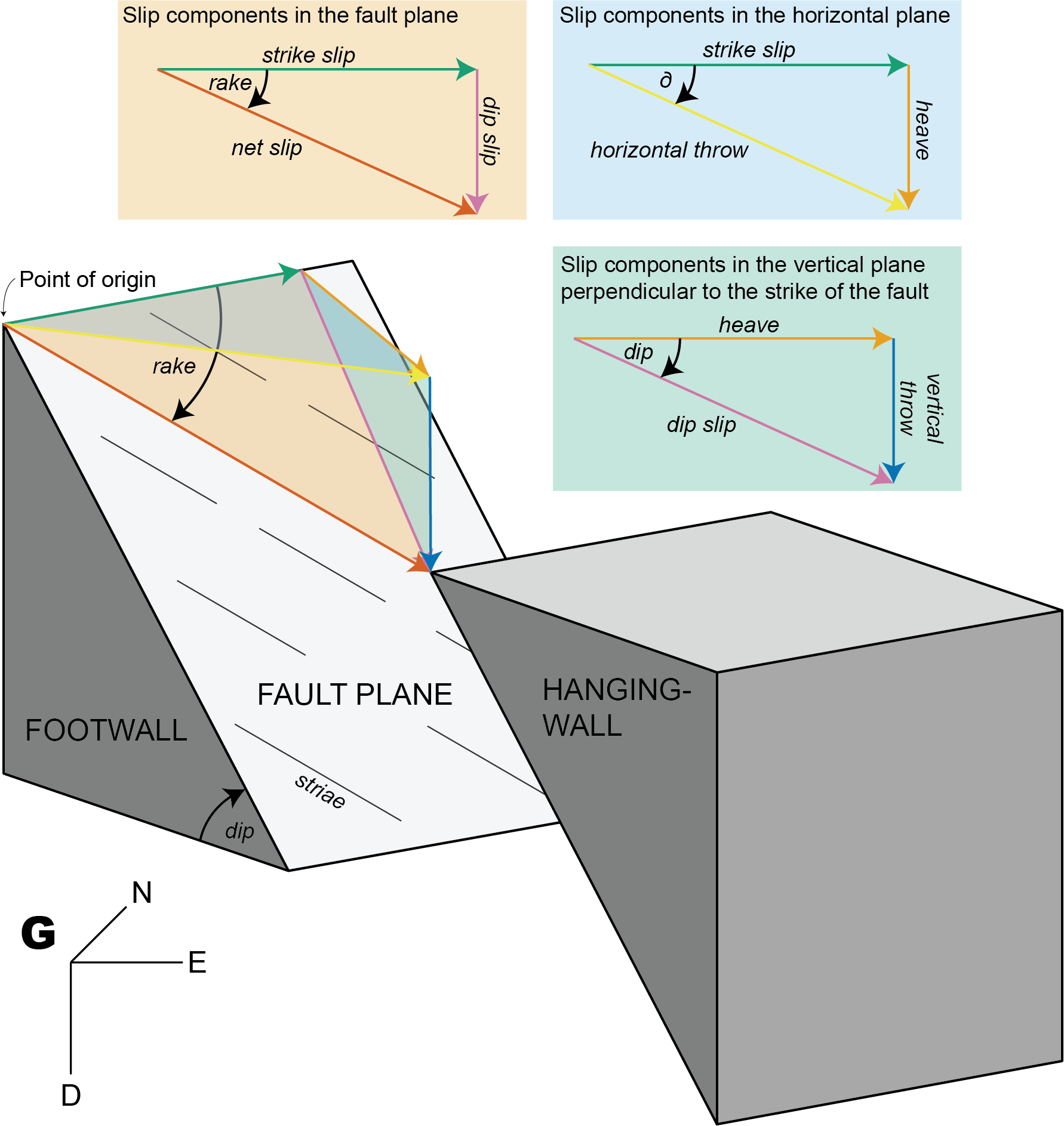
Get different components with trigonometry

1. Input: Fault orientation (dip angle, dip direction), shorteninig direction, and horizontal throw

Knowing the horizontal throw (e.g. from plate motion parameters), the remaining components of the displacements along a given fault are as follows.

$$\begin{equation}\delta = |\sigma_{\textrm{Hmax}} - (\textrm{dip direction}+90^{\circ})|\end{equation}$$

Slip components in the horizontal plane:

$$\begin{equation}\begin{split} f_\textrm{strike slip} & = |\cos{\delta} * f_\textrm{horizontal throw}|\\ f_\textrm{heave} & = \sqrt{f_\textrm{horizontal throw}^2 - f_\textrm{strike slip}^2} \end{split}\end{equation}$$

Slip components in the vertical plane perpendicular to the strike of the fault:

$$\begin{equation}\begin{split} f_\textrm{dip slip} &= \frac{f_\textrm{heave}}{cos{(\textrm{dip})}}\\ f_\textrm{vertical throw} &= \sqrt{f_\textrm{dip slip}^2 - f_\textrm{heave}^2} \end{split}\end{equation}$$

Slip components in the fault plane plane:

$$\begin{equation}\begin{split} f_\textrm{net slip} &= \sqrt{f_\textrm{strike slip}^2 + f_\textrm{dip slip}^2}\\ \textrm{rake} &= \arctan{\left(\frac{f_\textrm{dip slip}}{f_\textrm{strike slip}}\right)} \end{split}\end{equation}$$

Thus, the rake angle describes the ratio between the dip slip and the strike slip component.

Knowing the vertical throw (e.g. from thermochronology or petrology), the fault dip (?assumption), and the direction and amount of horizontal offset, the strike of the fault is as follows:

$$\begin{equation}\begin{split} f_\textrm{heave} &= f_\textrm{vertical throw} * \tan{(\textrm{dip})}\\ \delta &= \arcsin{\left(\frac{f_\textrm{heave}}{f_\textrm{horizontal throw}}\right)}\\ \textrm{strike} &= |\sigma_{\textrm{Hmax}} - \delta| \end{split}\end{equation}$$

Knowing the vertical throw (e.g. from thermochronology or petrology), the fault strike (geomorphology), and the direction and amount of horizontal offset, the dip of the fault is as follows:

$$\begin{equation}\begin{split} \delta &= |\sigma_{\textrm{Hmax}} - \textrm{strike}|\\ f_\textrm{heave} &= f_\textrm{horizontal throw} * \sin{\delta} \\ \textrm{dip} &= \arctan{\left(\frac{f_\textrm{heave}}{f_\textrm{vertical throw}}\right)} \end{split}\end{equation}$$

Knowing the vertical throw (e.g. from thermochronology or petrology) and the fault’s dip and rake, the horizontal offset, the horizontal throw, and the net-slip are as follows:

Fault displacement tensors

Each fault component is a vector describing its direction and length. For instance, the vector of the strike slip is:

$$\begin{equation} \vec{f_\text{strike slip}} = \begin{pmatrix} \lVert f_\textrm{strike-slip}\rVert \\ 0 \\ 0 \end{pmatrix} \end{equation}$$

Net slip vector

Net slip vector

$$\begin{equation} \vec{f_\text{net}} = \begin{pmatrix} \lVert f_\textrm{strike-slip}\rVert \\ \lVert f_\textrm{heave}\rVert \\ \lVert f_\textrm{vertical throw}\rVert \end{pmatrix} \end{equation}$$

fault_displacements(strikeslip = 2, verticalthrow = -5, heave = 3)

Principal displacement tensor

The Eigen values of $\mathsf{F}_{ij}$; represented as $\{ \vec{f_1}, \vec{f_2}, \vec{f_3} \}$ are referred to as the heave, strike slip, and vertical throw component, respectively. These orthonormal vectors define a orthogonal matrix, i.e. the principal displacement tensor $\mathsf{F}_\mathbb{F}$:

$$\begin{equation}\mathsf{F}_{\mathbb{F}} = {\begin{bmatrix} \lVert f_\textrm{heave}\rVert & 0 & 0\\ 0 & \lVert f_\textrm{strike-slip}\rVert & 0\\ 0 & 0 & \lVert f_\textrm{vertical throw}\rVert\end{bmatrix}}\end{equation}$$

The tensor $\mathsf{F}$ can also be defined by the magnitudes of the fault displacements:

Fu <- displacement_tensor(s = 2, v = -5, h = 3)
print(Fu)

##      [,1] [,2] [,3]
## [1,]    3    0    0
## [2,]    0    2    0
## [3,]    0    0   -5
## attr(,"class")
## [1] "matrix"  "array"   "ftensor"

Orientation tensor

Fault orientation tensor is defined by the fault plane’s location, orientation (dip direction and dip angle), and the fault’s slip (direction and magnitude):

$$\begin{equation}\mathsf{F}_{ij} = {\begin{bmatrix}f_{11} & f_{12} & f_{13}\\ f_{21} & f_{22} & f_{23}\\ f_{31} & f_{32} & f_{33}\end{bmatrix}}\end{equation}$$

Fg <- displacement_tensor(s = 2, v = -5, h = 3, dip_direction = 45)
print(Fg)

##         [,1]      [,2] [,3]
## [1,] 2.12132  1.414214    0
## [2,] 2.12132 -1.414214    0
## [3,] 0.00000  0.000000   -5
## attr(,"class")
## [1] "matrix"  "array"   "ftensor"

From Principal displacement tensor to Orientation tensor

Translation point of origin in $\mathsf{F_\mathbb{F}}$ into point of measurement and rotate into fault orientation $\mathsf{F}_\mathbb{FG}$

displacement_tensor_decomposition(Fg, dip_direction = 45)

## $displacements
##           dip    delta     rake verticalthrow horizontalthrow heave  dipslip
## [1,] 300.9638 56.30993 71.06818            -5        3.605551     3 5.830952
##      strikeslip  netslip
## [1,]          2 6.164414
## 
## $fault
## Fault object (n = 1):
## dip_direction           dip       azimuth        plunge         sense 
##      45.00000     300.96376     258.69007      54.20424      -1.00000 
## 
## $strain_tensor
##      [,1] [,2] [,3]
## [1,]  3.0 -1.5 -1.5
## [2,] -1.0  1.0 -1.0
## [3,]  2.5  2.5 15.0
## 
## $volumetric_strain
## [1] 19
## 
## $shear_strain
## [1] 5.196152

References

Angelier, J. (1979). Determination of the mean principal directions of stresses for a given fault population. Tectonophysics, 56(3–4), T17–T26. https://doi.org/10.1016/0040-1951(79)90081-7

Angelier, J. (1990). Inversion of field data in fault tectonics to obtain the regional stress—III. A new rapid direct inversion method by analytical means. Ceophys. J. Int, 103, 363–376. https://doi.org/10.1111/j.1365-246X.1990.tb01777.x

Lund, B., & Townend, J. (2007). Calculating horizontal stress orientations with full or partial knowledge of the tectonic stress tensor. Geophysical Journal International, 170(3), 1328–1335. https://doi.org/10.1111/j.1365-246X.2007.03468.x

Michael, A. J. (1984). Determination of stress from slip data: Faults and folds. Journal of Geophysical Research: Solid Earth, 89(B13), 11517–11526. https://doi.org/10.1029/JB089iB13p11517