7. Strain and Vorticity Analysis

Tobias Stephan

2025-10-03

library(structr)

Strain analysis (fabric analysis)

Import some R-phi data from elliptical strain markers

data(ramsay)
head(ramsay)
#>         R   phi
#> [1,] 1.24 35.96
#> [2,] 1.52 27.59
#> [3,] 1.33 36.91
#> [4,] 1.78 27.31
#> [5,] 1.51 17.73
#> [6,] 1.70 24.45

The mean mean strain ellipse (shape and orientation) of deformed elliptical objects as strain markers can be calculated by using the mean shape matrix and its eigenvalues (Shimamoto and Ikeda, 1976):

ramsay_mean <- mean_strain_ellipse(r = ramsay[, 1], phi = ramsay[, 2])
print(ramsay_mean)
#> $R
#> [1] 1.628138
#> 
#> $phi
#> [1] 25.73632
#> 
#> $R_CI
#> [1] 1.59275 1.66359
#> 
#> $phi_CI
#> [1] 24.71905 26.75180

The {structr} algorithm also calculates bootstrapped 95% confidence interval.

To visualize the distribution of the strain values, we can calculate densities in Rf-Phi space and plot them in a Rf/phi diagram:

Rphi_plot(r = ramsay[, 1], phi = ramsay[, 2])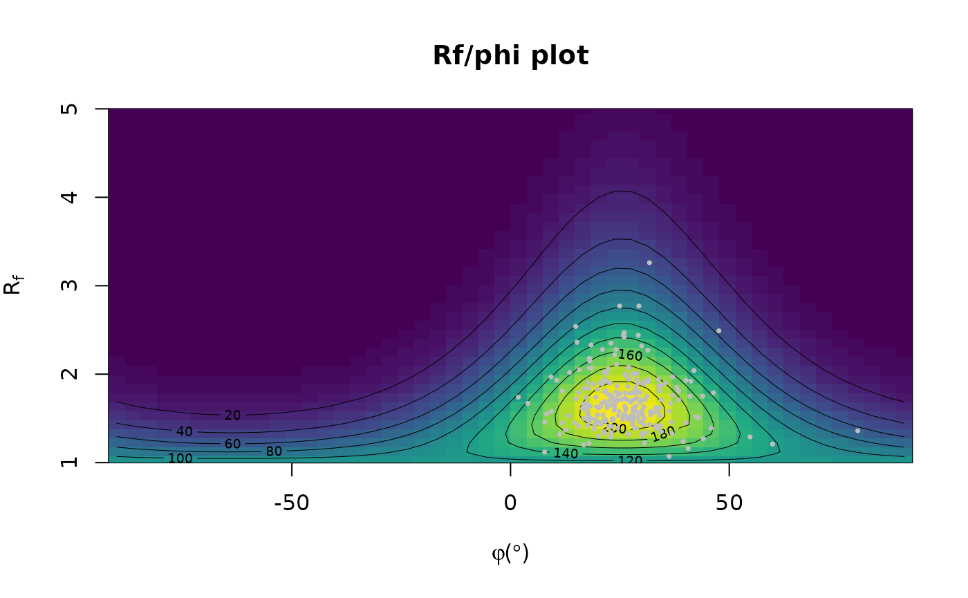

or in an Equidistant polar plot:

Rphi_polar_plot(ramsay[, 1], ramsay[, 2], proj = "eqd")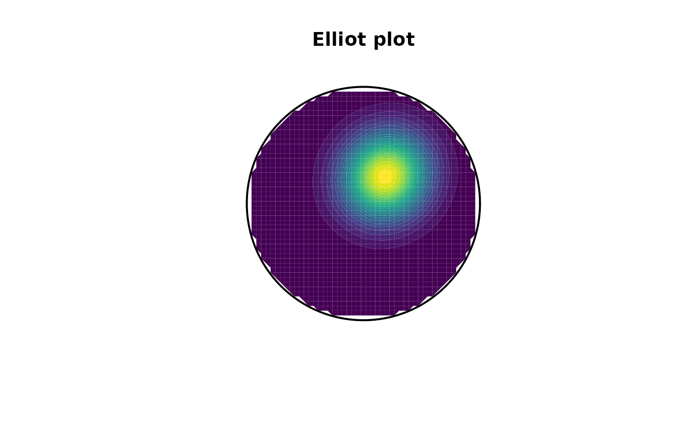

3D Strain

Three-dimensional strain data are expressed by the ratio of the magnitudes of the 3 principal strain axes of the strain ellipsoid, $X \geq Y \geq Z$. They can be represented in the Flinn diagram (linear of logarithmic axes)…

data("holst")
R_XY <- holst[, "R_XY"]
R_YZ <- holst[, "R_YZ"]

flinn_plot(R_XY, R_YZ, log = TRUE, col = "#B63679", pch = 16)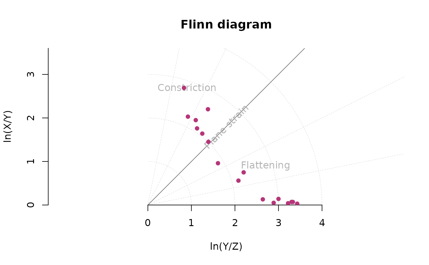

or the Hsü diagram using the natural octahedral unit strain $\bar{\epsilon}_s$ and the Lode parameter $\nu$

hsu_plot(R_XY, R_YZ, col = "#B63679", pch = 16)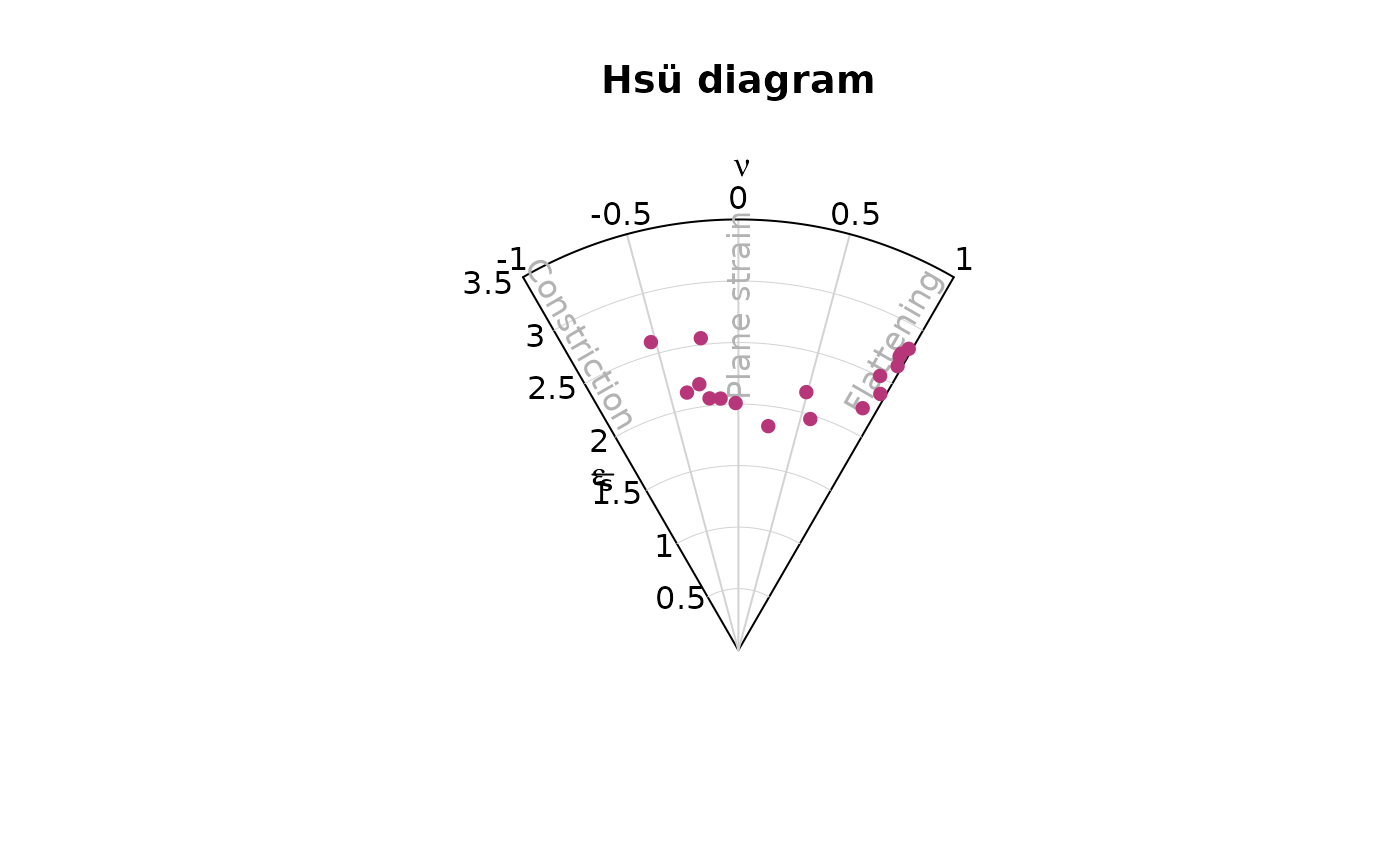

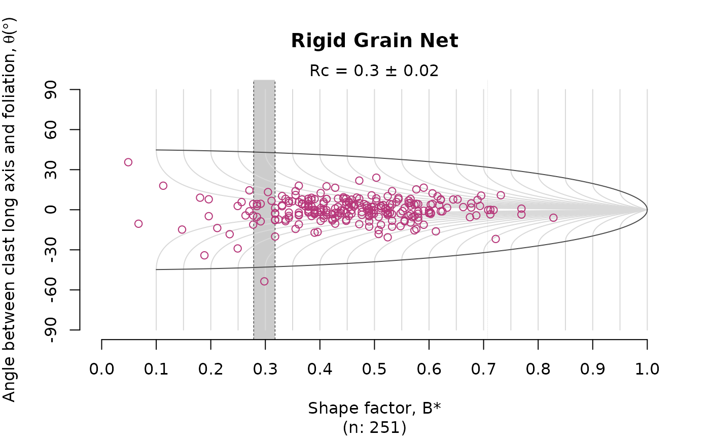
Vorticity analysis

The rigid grain net after (Jessup et al. 2007) plots the distribution the strain ratio (R) of orientation (phi) of porphyroclast over the theoretical distribution of tailless clasts. The plot estimates the critical threshold Rc marking the transition between the stable-sink position and infinitely rotating porphyroclasts. This threshold can be interpreted as the the mean kinematic vorticity number. Here the Rc is estimated using the bootstrap method described in Stephan et al. (2025).

# assuming the mean orientation resembles the foliation
theta <- tectonicr::circular_mean(ramsay[, 2]) - ramsay[, 2]

RGN_plot(r = ramsay[, 1], theta = theta, col = "#B63679")
title(main = "Rigid Grain Net")