Kamb counts and densities on the sphere
Usage
spherical_density(
  x,
  kamb = TRUE,
  FUN = exponential_kamb,
  ngrid = 128L,
  sigma = 3,
  vmf_hw = NULL,
  vmf_optimal = c("cross", "rot"),
  weights = NULL,
  upper.hem = FALSE,
  r = 1
)

stereo_density(
  x,
  kamb = TRUE,
  FUN = exponential_kamb,
  ngrid = 128L,
  sigma = 3,
  vmf_hw = NULL,
  vmf_optimal = c("cross", "rot"),
  weights = NULL,
  upper.hem = FALSE,
  r = 1,
  type = c("contour", "contour_filled", "image"),
  nlevels = 10L,
  col.palette = viridis,
  col = NULL,
  add = TRUE,
  col.params = list(),
  ...
)
Arguments
- x
Object of class
"line"or"plane"or'spherical.density'(for plotting only).- kamb
logical. Whether to use the von Mises-Fisher kernel density estimation (
FALSE) or Kamb's method (TRUE, the default).- FUN
density estimation function if
kamb=TRUE; one ofexponential_kamb()(the default), kamb_count, andschmidt_count().- ngrid
integer. Gridzise. 128 by default.
- sigma
numeric. Radius for Kamb circle used for counting. 3 by default.
- vmf_hw
numeric. Kernel bandwidth in degree.
- vmf_optimal
character. Calculates an optimal kernel bandwidth using the cross-validation algorithm (
'cross') or the rule-of-thumb ('rot') suggested by Garcia-Portugues (2013). Ignored whenvmf_hwis specified.- weights
(optional) numeric vector of length of
azi. The relative weight to be applied to each input measurement. The array will be normalized to sum to 1, so absolute value of theweightsdo not affect the result. Defaults toNULL- upper.hem
logical. Whether the projection is shown for upper hemisphere (
TRUE) or lower hemisphere (FALSE, the default).- r
numeric. radius of stereonet circle
- type
character. Type of plot:
'contour'for contour lines,'contour_filled'for filled contours, or'image'for a raster image.- nlevels
integer. Number of contour levels for plotting
- col.palette
a color palette function to be used to assign colors in the plot.
- col
colour(s) for the contour lines drawn. If
NULL, lines are color based oncol.palette.- add
logical. Whether the contours should be added to an existing plot.
- col.params
list. Arguments passed to
col.palette- ...
Value
list containing the stereographic x and coordinates of of the grid, the counts, and the density.
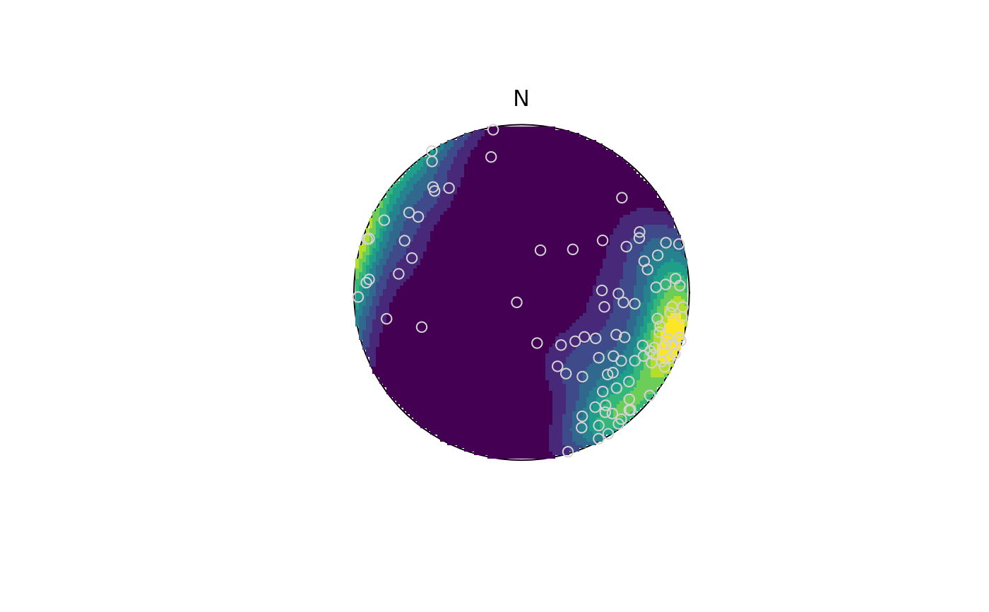
Examples
set.seed(20250411)
test <- rfb(100, mu = Line(120, 10), k = 5, A = diag(c(-1, 0, 1)))
test_densities <- spherical_density(x = test, ngrid = 100, sigma = 3, weights = runif(100))
stereo_density(test_densities, type = "image", add = FALSE)
stereo_point(test, col = "lightgrey", pch = 21)
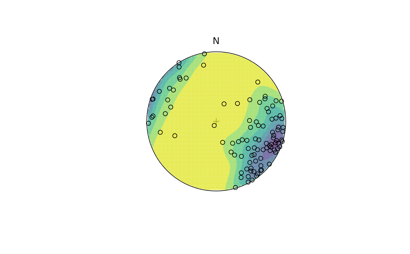
 stereo_density(test,
type = "contour_filled", add = FALSE,
col.params = list(direction = -1, begin = .05, end = .95, alpha = .75)
)
stereo_point(test, col = "black", pch = 21)
stereo_density(test,
type = "contour_filled", add = FALSE,
col.params = list(direction = -1, begin = .05, end = .95, alpha = .75)
)
stereo_point(test, col = "black", pch = 21)
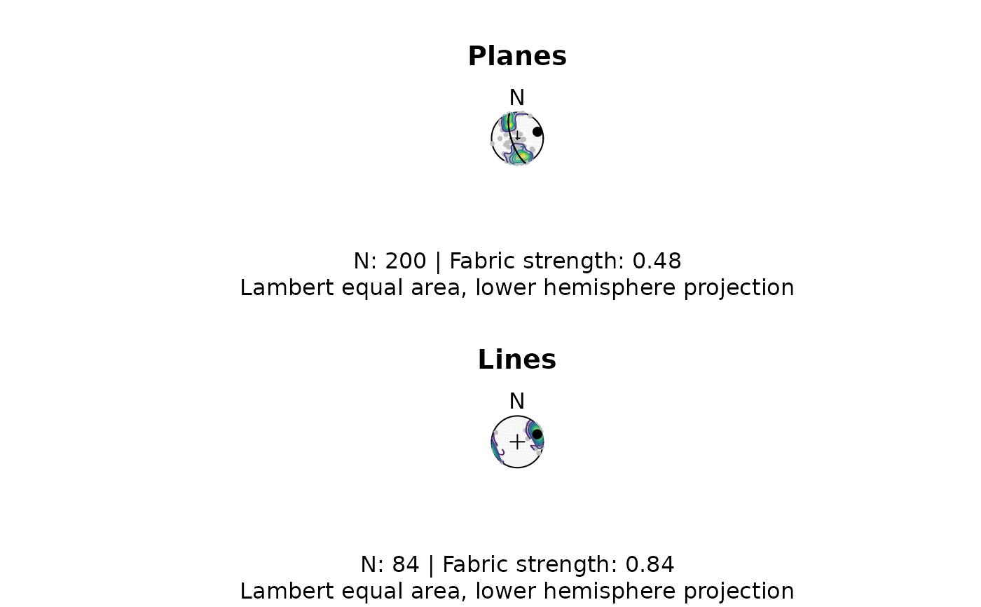
 # complete example:
par(mfrow = c(2, 1))
wp <- 6 / ifelse(is.na(example_planes$quality), 6, example_planes$quality)
my_planes <- Plane(example_planes$dipdir, example_planes$dip)
fabric_p <- or_shape_params(my_planes)$Vollmer["D"]
my_planes_eig <- or_eigen(my_planes)
stereoplot(guides = TRUE, col = "grey96")
stereo_point(my_planes, col = "grey", pch = 16, cex = .5)
stereo_density(my_planes, type = "contour", add = TRUE, weights = wp)
stereo_point(as.plane(my_planes_eig$vectors[3, ]), col = "black", pch = 16)
stereo_greatcircle(as.plane(my_planes_eig$vectors[3, ]), col = "black", pch = 16)
title(
main = "Planes",
sub = paste0(
"N: ", nrow(my_planes), " | Fabric strength: ", round(fabric_p, 2),
"\nLambert equal area, lower hemisphere projection"
)
)
my_lines <- Line(example_lines$trend, example_lines$plunge)
wl <- 6 / ifelse(is.na(example_lines$quality), 6, example_lines$quality)
fabric_l <- or_shape_params(my_lines)$Vollmer["D"]
stereoplot(guides = TRUE, col = "grey96")
stereo_point(my_lines, col = "grey", pch = 16, cex = .5)
stereo_density(my_lines, type = "contour", add = TRUE, weights = wl)
stereo_point(v_mean(my_lines, w = wl), col = "black", pch = 16)
title(
main = "Lines",
sub = paste0(
"N: ", nrow(my_lines), " | Fabric strength: ", round(fabric_l, 2),
"\nLambert equal area, lower hemisphere projection"
)
)
# complete example:
par(mfrow = c(2, 1))
wp <- 6 / ifelse(is.na(example_planes$quality), 6, example_planes$quality)
my_planes <- Plane(example_planes$dipdir, example_planes$dip)
fabric_p <- or_shape_params(my_planes)$Vollmer["D"]
my_planes_eig <- or_eigen(my_planes)
stereoplot(guides = TRUE, col = "grey96")
stereo_point(my_planes, col = "grey", pch = 16, cex = .5)
stereo_density(my_planes, type = "contour", add = TRUE, weights = wp)
stereo_point(as.plane(my_planes_eig$vectors[3, ]), col = "black", pch = 16)
stereo_greatcircle(as.plane(my_planes_eig$vectors[3, ]), col = "black", pch = 16)
title(
main = "Planes",
sub = paste0(
"N: ", nrow(my_planes), " | Fabric strength: ", round(fabric_p, 2),
"\nLambert equal area, lower hemisphere projection"
)
)
my_lines <- Line(example_lines$trend, example_lines$plunge)
wl <- 6 / ifelse(is.na(example_lines$quality), 6, example_lines$quality)
fabric_l <- or_shape_params(my_lines)$Vollmer["D"]
stereoplot(guides = TRUE, col = "grey96")
stereo_point(my_lines, col = "grey", pch = 16, cex = .5)
stereo_density(my_lines, type = "contour", add = TRUE, weights = wl)
stereo_point(v_mean(my_lines, w = wl), col = "black", pch = 16)
title(
main = "Lines",
sub = paste0(
"N: ", nrow(my_lines), " | Fabric strength: ", round(fabric_l, 2),
"\nLambert equal area, lower hemisphere projection"
)
)