3. Plotting trajectories of theoretic stress directions

This vignette teaches you how to plot the trajectories of the predicted stress directions.

library(tectonicr)
library(ggplot2) # load ggplot library
library(sf)

Equivalent rotations

Relative plate motions from a set of (global) plate motions can be retrieved by transforming the set of the Euler rotations parameters to equivalent rotations.

The NUVEL1 data set offers the global plate motions relative to the Pacific plate (DeMets et al. 1990). In order to extract the plate motions between two other plates (e.g. all plates relative to Eurasia), one has to transform the rotations in to a new, equivalent reference system (i.e. all rotation with respect to (wrt.) Eurasia).

In tectonicr this can be done with equivalent_rotation():

data("nuvel1")
nuvel1.eu <- equivalent_rotation(nuvel1, fixed = "eu")
head(nuvel1.eu)
#>    plate.rot       lat        lon      angle plate.fix
#> af        af  21.22431  -20.25390 0.12839397        eu
#> an        an  37.85378   77.54263 0.05402503        eu
#> ar        ar  24.77897   14.14654 0.51993229        eu
#> au        au  15.28437   40.87794 0.71935116        eu
#> ca        ca -50.85213  -50.33611 0.12128773        eu
#> co        co  19.84642 -115.85295 1.36455727        eu

Alternatively, the PB2002 model by Bird (2003) is also provided as an ready-to use example dataset for global plate motions.

data("pb2002")
pb2002.eu <- equivalent_rotation(pb2002, fixed = "eu")
head(pb2002.eu)
#>    plate.rot       lat       lon      angle plate.fix
#> af        af  21.21561 -20.26957 0.12277039        eu
#> am        am  22.31703 -73.10293 0.09095410        eu
#> an        an  37.88026  77.51306 0.05166503        eu
#> ap        ap -34.90145 -75.14215 0.42687654        eu
#> ar        ar  28.26668  11.83784 0.53270842        eu
#> as        as -27.83397  95.48900 0.27101254        eu

Plotting Pole of Rotation Grids

To visualize the theoretical trajectories of the direction of $\sigma_{Hmax}$ (great circles, small circles, and loxodomes), we need to transform the locations from the geographical coordinate system into the PoR coordinate system. The transformations are done through the function functions geographical_to_PoR() and PoR_to_geographical(). They are the base of the functions eulerpole_smallcircles(), eulerpole_greatcircles(), and eulerpole_loxodromes() that allow to draw the theoretical trajectories in geographical coordinates.

Small Circles

Function eulerpole_smallcircles(x, gridsize) returns small circles as as simple feature(sf) by giving a data.frame of the PoR coordinates in lat and lon (x) and the number of small circles (n).

For example the small circles around the pole of the relative motion of the Indian plate relative to the Eurasian plate (transformed from the from the NUVEL1 model).

por <-
  subset(nuvel1.eu, nuvel1$plate.rot == "in") # India relative to Eurasia

The returnclass option in eulerpole_smallcircles() provides the output types "sf" (for a simple feature) and "sp" (Spatial* object) for the small circles.

To eventually plot the small circles with ggplot, I recommend to extract a sf feature and plot the it with geom_sf():

por.sm <- eulerpole_smallcircles(por)
data("plates") # load plate boundary data set
# world <- rnaturalearth::ne_countries(scale = "small", returnclass = "sf")

ggplot() +
  # geom_sf(data = world, alpha = .5) +
  geom_sf(
    data = plates,
    color = "red",
    alpha = .5
  ) +
  labs(title = "India relative to Eurasia", subtitle = "source: NUVEL1") +
  geom_sf(
    data = por.sm,
    aes(lty = "small circles"),
    color = "darkblue", fill = NA,
    alpha = .5
  ) +
  geom_point(
    data = por,
    aes(lon, lat),
    shape = 21,
    colour = "lightblue",
    size = 2,
    fill = "darkblue",
    stroke = 1
  ) +
  geom_point(
    data = euler,
    aes(lon + 180, -lat),
    shape = 21,
    colour = "lightblue",
    size = 2,
    fill = "darkblue",
    stroke = 1
  ) +
  coord_sf(default_crs = "WGS84", crs = sf::st_crs("ESRI:54030"))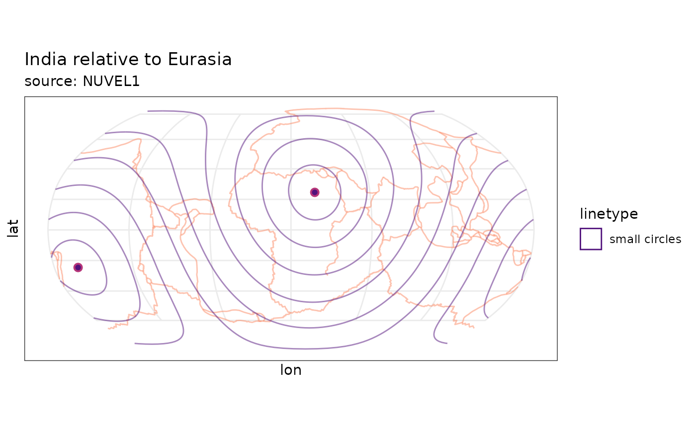

Predicted SHmax trajectories that are small circles around the In-Eu pole of rotation.

Great Circles

Great circles are lines that cut the small circles at 90 $^{\circ}$ and the PoR. Function eulerpole_greatcircles(x, n) returns great circles as sf object by giving a data.frame of the Pole of Rotation (PoR) coordinates in lat and lon (x) and the number of great circles n, or the great circle angles (360/d).

por.gm <- eulerpole_greatcircles(por)

ggplot() +
  # geom_sf(data = world, alpha = .5) +
  geom_sf(
    data = plates,
    color = "red",
    alpha = .5
  ) +
  labs(title = "India relative to Eurasia", subtitle = "source: NUVEL1") +
  geom_sf(
    data = por.sm,
    aes(lty = "small circles"),
    color = "darkblue",
    alpha = .5
  ) +
  geom_sf(
    data = por.gm,
    aes(lty = "great circles"),
    color = "darkblue"
  ) +
  geom_point(
    data = por,
    aes(lon, lat),
    shape = 21,
    colour = "lightblue",
    size = 2,
    fill = "darkblue",
    stroke = 1
  ) +
  geom_point(
    data = por,
    aes(lon + 180, -lat),
    shape = 21,
    colour = "lightblue",
    size = 2,
    fill = "darkblue",
    stroke = 1
  ) +
  coord_sf(default_crs = "WGS84", crs = sf::st_crs("ESRI:54030"))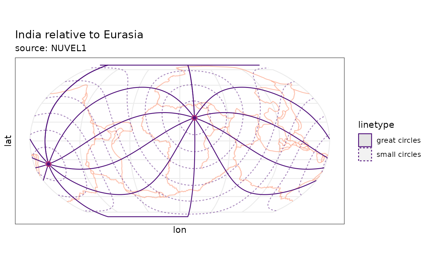

Predicted SHmax trajectories that are great circles passing through the In-Eu pole of rotation.

Loxodromes

Loxodrome (also called Rhumb Line) is a curve cutting the small circles at a constant angle. Thus, small and great circles are 0 $^{\circ}$ and 90 $^{\circ}$ loxodromes, respectively.

Function eulerpole_loxodromes(x, n) returns loxodromes as sf object by giving a data.frame of the PoR coordinates in lat and lon (x) and the angle between the loxodromes, the direction, and the sense.

por.ld <- eulerpole_loxodromes(x = por, angle = 45, n = 10, cw = TRUE)

ggplot() +
  labs(title = "India relative to Eurasia", subtitle = "source: NUVEL1") +
  # geom_sf(data = world, alpha = .5) +
  geom_sf(
    data = plates,
    color = "red",
    alpha = .5
  ) +
  geom_sf(
    data = por.sm,
    aes(lty = "small circles"),
    color = "darkblue",
    alpha = .5
  ) +
  geom_sf(
    data = por.ld,
    aes(lty = "clockwise loxodromes"),
    color = "darkblue"
  ) +
  geom_point(
    data = por,
    aes(lon, lat),
    shape = 21,
    colour = "lightblue",
    size = 2,
    fill = "darkblue",
    stroke = 1
  ) +
  geom_point(
    data = por,
    aes(lon + 180, -lat),
    shape = 21,
    colour = "lightblue",
    size = 2,
    fill = "darkblue",
    stroke = 1
  ) +
  coord_sf(default_crs = "WGS84", crs = sf::st_crs("ESRI:54030"))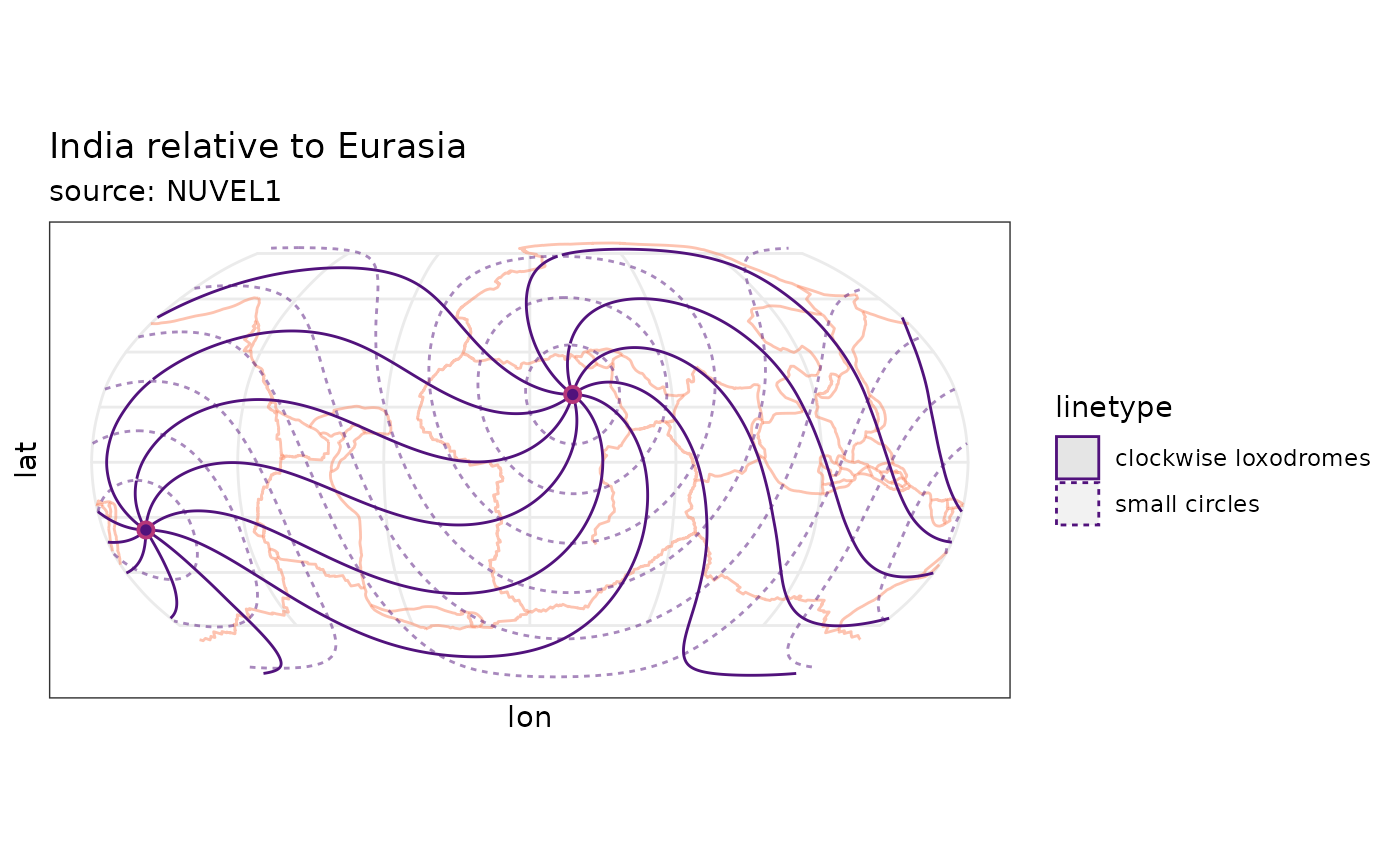

Predicted SHmax trajectories that are 45-degree loxodromes circles directed towards the In-Eu pole of rotation.

References

Bird, Peter. 2003. “An Updated Digital Model of Plate Boundaries” Geochemistry, Geophysics, Geosystems 4 (3). doi: 10.1029/2001gc000252.

DeMets, C., R. G. Gordon, D. F. Argus, and S. Stein. 1990. “Current Plate Motions” Geophysical Journal International 101 (2): 425–78. doi: 10.1111/j.1365-246x.1990.tb06579.x.