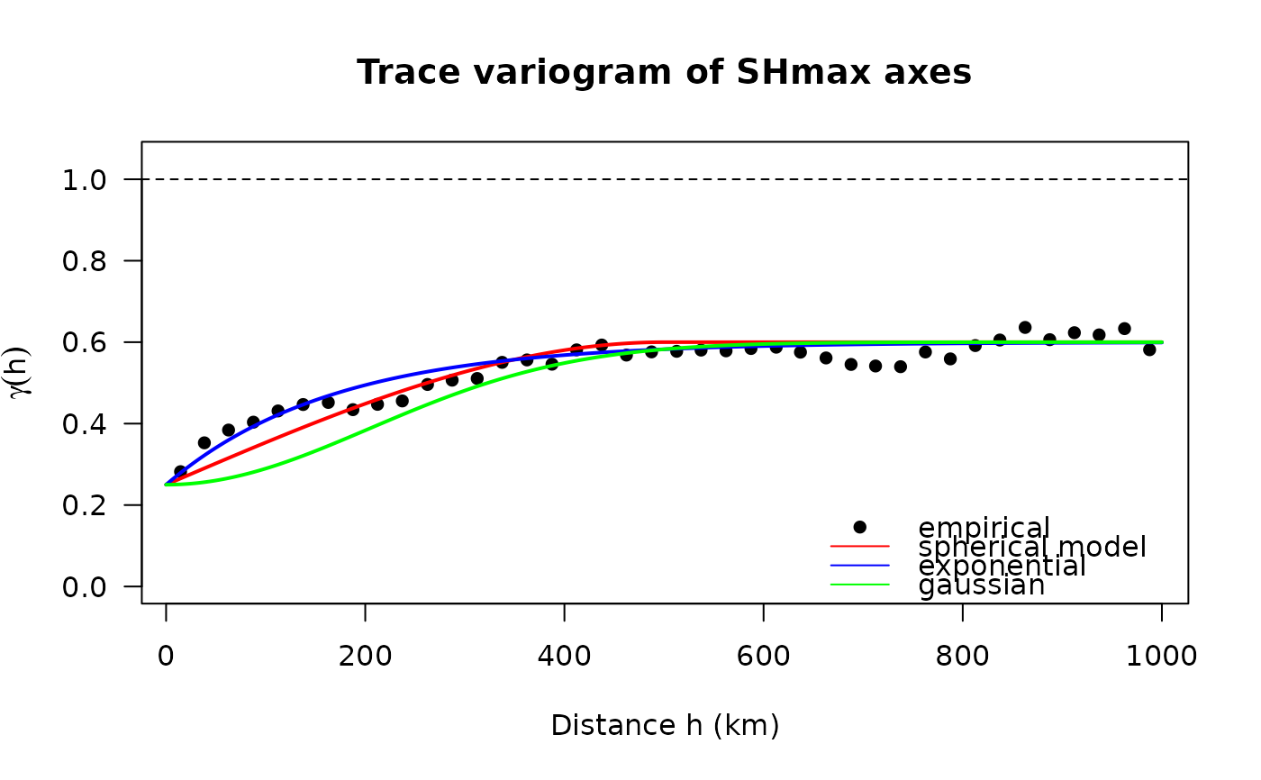
Empirical trace variogram of axial data, for choosing the model
Source:R/interpolation_krige.R
variogram_axial.RdBins the empirical variogram \(\gamma(h) = \text{mean}(||T_i - T_j||_F^2)\), where
T = ortensor2d(a, norm = TRUE) for each axis. For axes this equals
\(\text{mean}(1 - \cos(2 (a_i - a_j)))\). Use it to choose nugget and range_km
for circular_krige().
Usage
variogram_axial(x, breaks = seq(0, 500, 50))Examples
v <- variogram_axial(san_andreas, breaks = seq(0, 1000, 25))
v <- v[!is.na(v$gamma), ] # drop empty bins

plot(v$lag, v$gamma, pch = 16, las = 1,
  xlab = "Distance h (km)", ylab = expression(gamma(h)),
  ylim = c(0, 1.05), main = "Trace variogram of SHmax axes")
abline(h = 1, lty = 2) # sill: trace of a unit tensors

h <- seq(0, 1000, length.out = 300)
lines(h, krige_gamma(h, model = "spherical",
  nugget = 0.25, range_km = 500, sill = 0.6),
  col = "red", lwd = 2)#'
lines(h, krige_gamma(h, model = "exponential",
  nugget = 0.25, range_km = 500, sill = 0.6),
  col = "blue", lwd = 2)
lines(h, krige_gamma(h, model = "gaussian",
  nugget = 0.25, range_km = 500, sill = 0.6),
  col = "green", lwd = 2)
legend("bottomright", legend = c("empirical", "spherical model", "exponential", "gaussian"),
 pch = c(16, NA, NA, NA), lty = c(NA, 1, 1, 1), col = c("black", "red", "blue", "green"), bty = "n")