Adaptive kernel density estimates

Modification of ggplot2::stat_density() for kernel density estimates using a combination of the Botev (2010) bandwidth selector and the Abramson (1982) adaptive kernel bandwidth modifier.

Usage

stat_aKDE(
  mapping = NULL,
  data = NULL,
  stat = "DensityAdaptive",
  geom = "area",
  position = "stack",
  ...,
  from = NA,
  to = NA,
  bw = NA,
  adjust = 1,
  kernel = "gaussian",
  n = 512,
  adaptive = TRUE,
  na.rm = FALSE,
  bounds = c(-Inf, Inf),
  show.legend = NA,
  orientation = NA,
  inherit.aes = TRUE
)

geom_aKDE(
  mapping = NULL,
  data = NULL,
  stat = "DensityAdaptive",
  position = "identity",
  ...,
  na.rm = FALSE,
  orientation = NA,
  show.legend = NA,
  inherit.aes = TRUE,
  outline.type = "upper"
)

Source

Algorithm for adaptive kernel is modified from IsoplotR. The algorithm for the optimal kernel bandwidth is from provenance::botev().

Arguments

mapping

Set of aesthetic mappings created by aes(). If specified and inherit.aes = TRUE (the default), it is combined with the default mapping at the top level of the plot. You must supply mapping if there is no plot mapping.

data

The data to be displayed in this layer. There are three options:

If NULL, the default, the data is inherited from the plot data as specified in the call to ggplot().

A data.frame, or other object, will override the plot data. All objects will be fortified to produce a data frame. See fortify() for which variables will be created.

A function will be called with a single argument, the plot data. The return value must be a data.frame, and will be used as the layer data. A function can be created from a formula (e.g. ~ head(.x, 10)).

geom, stat

Use to override the default connection between geom_density() and stat_density().

position

Position adjustment, either as a string naming the adjustment (e.g. "jitter" to use position_jitter), or the result of a call to a position adjustment function. Use the latter if you need to change the settings of the adjustment.

...

Other arguments passed on to layer(). These are often aesthetics, used to set an aesthetic to a fixed value, like colour = "red" or size = 3. They may also be parameters to the paired geom/stat.

from, to

the left and right-most points of the grid at which the density is to be estimated

bw

the bandwidth of the KDE. If NULL, bw will be calculated automatically using the algorithm by Botev et al. (2010).

adjust

A multiplicate bandwidth adjustment. This makes it possible to adjust the bandwidth while still using the a bandwidth estimator. For example, adjust = 1/2 means use half of the default bandwidth.

kernel

Kernel. See list of available kernels in density().

n

number of equally spaced points at which the density is to be estimated, should be a power of two, see density() for details

adaptive

logical flag controlling if the adaptive KDE modifier of Abramson (1982) is used

na.rm

If FALSE, the default, missing values are removed with a warning. If TRUE, missing values are silently removed.

bounds

Known lower and upper bounds for estimated data. Default c(-Inf, Inf) means that there are no (finite) bounds. If any bound is finite, boundary effect of default density estimation will be corrected by reflecting tails outside bounds around their closest edge. Data points outside of bounds are removed with a warning.

show.legend

logical. Should this layer be included in the legends? NA, the default, includes if any aesthetics are mapped. FALSE never includes, and TRUE always includes. It can also be a named logical vector to finely select the aesthetics to display.

orientation

The orientation of the layer. The default (NA) automatically determines the orientation from the aesthetic mapping. In the rare event that this fails it can be given explicitly by setting orientation to either "x" or "y". See the Orientation section for more detail.

inherit.aes

If FALSE, overrides the default aesthetics, rather than combining with them. This is most useful for helper functions that define both data and aesthetics and shouldn't inherit behaviour from the default plot specification, e.g. borders().

outline.type

Type of the outline of the area; "both" draws both the upper and lower lines, "upper"/"lower" draws the respective lines only. "full" draws a closed polygon around the area.

Examples

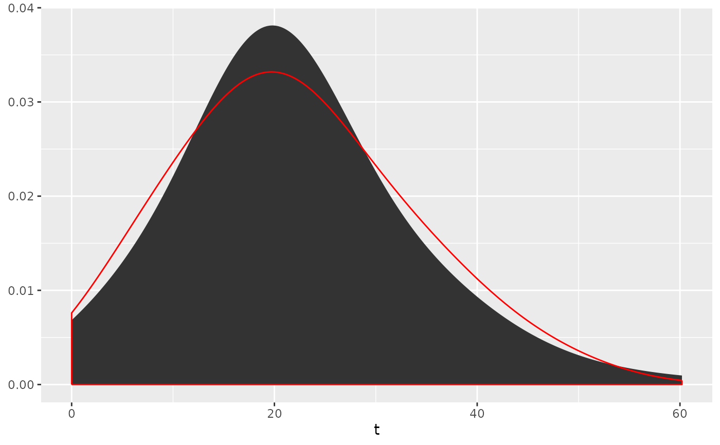
data("sample")
example <- age_ICP(sample, zeta = c(0.1188, 0.0119))
# IsoplotR::kde(example$ages$t)
ggplot2::ggplot(data = example$ages, mapping = ggplot2::aes(x = t)) +
  stat_aKDE(adaptive = TRUE) +
  stat_aKDE(adaptive = FALSE, color = "red", fill = NA)
#> Warning: Removed 3 rows containing non-finite outside the scale range
#> (`stat_density_adaptive()`).
#> Warning: Removed 3 rows containing non-finite outside the scale range
#> (`stat_density_adaptive()`).


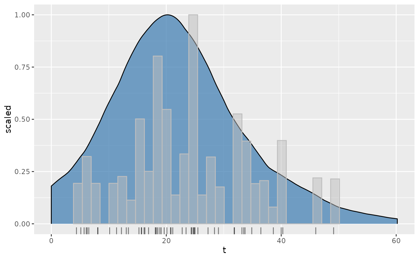
ggplot2::ggplot(
  data = example$ages,
  mapping = ggplot2::aes(x = t, weight = t / st)
) +
  geom_aKDE(
    ggplot2::aes(y = ggplot2::after_stat(scaled)),
    kernel = "epanechnikov", fill = "steelblue", alpha = .75
  ) +
  ggplot2::geom_histogram(
    ggplot2::aes(y = ggplot2::after_stat(ncount)),
    color = "grey", fill = "grey", alpha = .5
  ) +
  ggplot2::geom_rug(alpha = 0.5)
#> Warning: Removed 3 rows containing non-finite outside the scale range
#> (`stat_density_adaptive()`).
#> `stat_bin()` using `bins = 30`. Pick better value with `binwidth`.
#> Warning: Removed 3 rows containing non-finite outside the scale range (`stat_bin()`).